clear all
use https://sscc.wisc.edu/sscc/pubs/real_world_tables/table1a3 Table 1 with Tests to Compare Groups
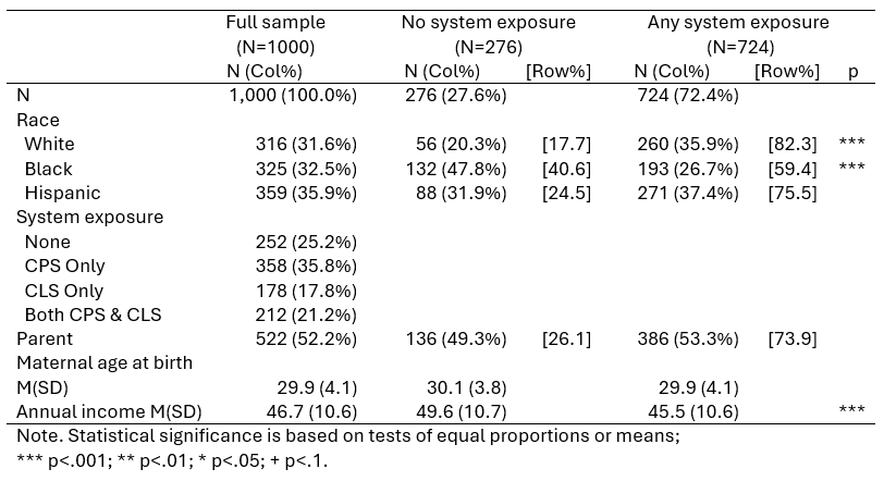
This is our final Table 1 and I saved the best for last, or at least the most complicated. Once again we have descriptive statistics, but this time there are two actual groups (“No system exposure” vs. “Any system exposure”) and we want to compare them. For indicator variables we want to run a proportion test, and this includes the indicator variables implied by the categorical variables (i.e. we want to test if the proportion of the “No” group that is White is equal to the proportion of the “Any” group that is White.) For quantitative variables we want to run a t-test for equal means. We also want to include row percentages.
Note that the “System exposure” categorical variable is what defines “No system exposure” vs. “Any system exposure”. “Any” includes “CPS Only”, “CLS Only” and “Both CPS & CLS.” Thus there’s no point in reporting descriptive statistics for “System exposure” across the two subgroups.
3.1 Setting Up
Load the data with:
Take a moment to look it over and identify the variable names. Yes, it’s the same data as in the first chapter.
3.2 Running Tests using dtable
The dtable command comes close to doing the tests you want if you just add the tests option to by(any):
dtable i.race i.exposure i.parent age income, by(any, tests)note: using test pearson across levels of any for race, exposure, and parent.
note: using test regress across levels of any for age and income.
----------------------------------------------------------------------------------
any
0 1 Total Test
----------------------------------------------------------------------------------
N 276 (27.6%) 724 (72.4%) 1,000 (100.0%)
Race
White 56 (20.3%) 260 (35.9%) 316 (31.6%) <0.001
Black 132 (47.8%) 193 (26.7%) 325 (32.5%)
Hispanic 88 (31.9%) 271 (37.4%) 359 (35.9%)
System exposure
None 276 (100.0%) 0 (0.0%) 276 (27.6%) <0.001
CPS Only 0 (0.0%) 290 (40.1%) 290 (29.0%)
CLS Only 0 (0.0%) 196 (27.1%) 196 (19.6%)
Both CPS & CLS 0 (0.0%) 238 (32.9%) 238 (23.8%)
Parent
No 140 (50.7%) 338 (46.7%) 478 (47.8%) 0.253
Yes 136 (49.3%) 386 (53.3%) 522 (52.2%)
Maternal age at birth M(SD) 30.052 (3.810) 29.880 (4.176) 29.928 (4.077) 0.551
Annual income M(SD) 49.621 (10.661) 45.529 (10.304) 46.658 (10.558) <0.001
----------------------------------------------------------------------------------For categorical variables, what it describes as a “pearson” test is a chi-squared test (compare tab parent any, chi2). Unfortunately that’s not what we want. The “regress” test comes down to a t-test when there are just two groups (compare ttest age, by(any)). That is what we want, but we since can’t use tests and get the proportion tests we want we’ll do the mean tests “by hand” too.
To get the collection you actually want to start with, remove the tests option.
dtable i.race i.exposure i.parent age income, by(any)
---------------------------------------------------------------------------
                                                  any
                                   0               1             Total
---------------------------------------------------------------------------
N                               276 (27.6%)     724 (72.4%)  1,000 (100.0%)
Race
  White                          56 (20.3%)     260 (35.9%)     316 (31.6%)
  Black                         132 (47.8%)     193 (26.7%)     325 (32.5%)
  Hispanic                       88 (31.9%)     271 (37.4%)     359 (35.9%)
System exposure
  None                         276 (100.0%)        0 (0.0%)     276 (27.6%)
  CPS Only                         0 (0.0%)     290 (40.1%)     290 (29.0%)
  CLS Only                         0 (0.0%)     196 (27.1%)     196 (19.6%)
  Both CPS & CLS                   0 (0.0%)     238 (32.9%)     238 (23.8%)
Parent
  No                            140 (50.7%)     338 (46.7%)     478 (47.8%)
  Yes                           136 (49.3%)     386 (53.3%)     522 (52.2%)
Maternal age at birth M(SD)  30.052 (3.810)  29.880 (4.176)  29.928 (4.077)
Annual income M(SD)         49.621 (10.661) 45.529 (10.304) 46.658 (10.558)
---------------------------------------------------------------------------
Note the structure:
collect layout
Collection: DTable
      Rows: var
   Columns: any#result
   Table 1: 15 x 3

---------------------------------------------------------------------------
                                                  any
                                   0               1             Total
---------------------------------------------------------------------------
N                               276 (27.6%)     724 (72.4%)  1,000 (100.0%)
Race
  White                          56 (20.3%)     260 (35.9%)     316 (31.6%)
  Black                         132 (47.8%)     193 (26.7%)     325 (32.5%)
  Hispanic                       88 (31.9%)     271 (37.4%)     359 (35.9%)
System exposure
  None                         276 (100.0%)        0 (0.0%)     276 (27.6%)
  CPS Only                         0 (0.0%)     290 (40.1%)     290 (29.0%)
  CLS Only                         0 (0.0%)     196 (27.1%)     196 (19.6%)
  Both CPS & CLS                   0 (0.0%)     238 (32.9%)     238 (23.8%)
Parent
  No                            140 (50.7%)     338 (46.7%)     478 (47.8%)
  Yes                           136 (49.3%)     386 (53.3%)     522 (52.2%)
Maternal age at birth M(SD)  30.052 (3.810)  29.880 (4.176)  29.928 (4.077)
Annual income M(SD)         49.621 (10.661) 45.529 (10.304) 46.658 (10.558)
---------------------------------------------------------------------------
Like with Table 1 (A), the level of result that’s actually being used is _dtable_stats.
3.3 Adding Statistics to the Collection
You need to add two things to this collection: row percentages, and stars indicating where there are significant differences. Both of these need to be calculated for every row in the table other than N, including each level of the categorical variables. This clearly calls for some loops. We’ll talk about each of the loop components before putting them all together and running them
For the categorical variables, the loop structure will be:
foreach var in race parent {
    levelsof `var', local(levels)
    foreach level of local levels {
This first loops over the categorical variables (race and parent). It then identifies the levels of the variable being used and loops over them. The current variable is stored in the macro `var' and the current level of that variable is stored in the macro `level'.
To calculate the row percentages, recall that the mean of an indicator variable is the proportion of observations that have a one for that variable. Thus sum any will give you the row proportion for the “Any” group. The easy way to get the row proportion for the “No” group is sum 0.any, where 0.any is an automatically-generated indicator for any==0. To identify the subgroup of interest, use `level'.`var'. This is an automatically-generated indicator for `var'==`level'. Thus the complete code for calculating the row proportions will be:
sum any if `level'.`var'and:
sum 0.any if `level'.`var'To put this in the collection, use collect get. Since you want row percentages rather than proportions, get r(mean) and multiply it by 100. The result needs to be tagged with the appropriate level of any as well as the appropriate row, which is again `level'.`var'. collect get gets the results of the most recent command, so the combined code is:
sum any if `level'.`var'
collect get rowpct=r(mean)*100, tag(any[1] var[`level'.`var'])

sum 0.any if `level'.`var'
collect get rowpct=r(mean)*100, tag(any[0] var[`level'.`var'])
Next comes the proportion test. You can’t use factor syntax like 0.race with prtest, so you need to create an indicator for “the observation is part of the group of interest.” When you’re done with it, drop it so you can create a new version for the next group.
The result to get for the collection is the p-value. The stars will go after the rightmost column, which is any[1], so you’ll need to tag the result with that as well as var[`level'.`var']
gen grp = (`var'==`level')
prtest grp, by(any)
collect get r(p), tag(any[1] var[`level'.`var'])
drop grp
Putting it all together (with a few strategically placed quietly: prefixes just to save space in this web book), you get:
foreach var in race parent {
    levelsof `var', local(levels)
    foreach level of local levels {

        quietly: sum any if `level'.`var'
        collect get rowpct=r(mean)*100, tag(any[1] var[`level'.`var'])

        quietly: sum 0.any if `level'.`var'
        collect get rowpct=r(mean)*100, tag(any[0] var[`level'.`var'])

        gen grp = (`var'==`level')
        quietly: prtest grp, by(any)
        collect get r(p), tag(any[1] var[`level'.`var'])
        drop grp
    }
}
0 1 2
0 1Next is the continuous variables. The process is similar, but simpler since there’s no need to deal with individual levels of the variables:
foreach var in age income {
    quietly: ttest `var', by(any)
    collect get r(p), tag(any[1] var[`var'])
}
Now you have all the results you need in your collection, and you just need a layout so you can see them all. The new stuff all goes in columns, so the row is still just var. The statistics collected by dtable are in result[dtable_stats]; add to them the results rowpct and p you collected. Also, you want the column for the full sample to come first, so specify the levels of any in that order:
collect layout (var) (any[.m 0 1]#result[_dtable_stats rowpct p])
Collection: DTable
      Rows: var
   Columns: any[.m 0 1]#result[_dtable_stats rowpct p]
   Table 1: 15 x 6

-----------------------------------------------------------------------------------------------
                                                            any
                                 Total                 0                         1
-----------------------------------------------------------------------------------------------
N                            1,000 (100.0%)     276 (27.6%)            724 (72.4%)
Race
  White                         316 (31.6%)      56 (20.3%) 17.722     260 (35.9%) 82.278 0.000
  Black                         325 (32.5%)     132 (47.8%) 40.615     193 (26.7%) 59.385 0.000
  Hispanic                      359 (35.9%)      88 (31.9%) 24.513     271 (37.4%) 75.487 0.102
System exposure
  None                          276 (27.6%)    276 (100.0%)               0 (0.0%)
  CPS Only                      290 (29.0%)        0 (0.0%)            290 (40.1%)
  CLS Only                      196 (19.6%)        0 (0.0%)            196 (27.1%)
  Both CPS & CLS                238 (23.8%)        0 (0.0%)            238 (32.9%)
Parent
  No                            478 (47.8%)     140 (50.7%) 29.289     338 (46.7%) 70.711 0.253
  Yes                           522 (52.2%)     136 (49.3%) 26.054     386 (53.3%) 73.946 0.253
Maternal age at birth M(SD)  29.928 (4.077)  30.052 (3.810)         29.880 (4.077)        0.551
Annual income M(SD)         46.658 (10.558) 49.621 (10.661)        45.529 (10.558)        0.000
-----------------------------------------------------------------------------------------------
You don’t really want the p-values in the table though, just stars if the difference is significant. You’re probably used to attaching stars to something else in your tables, but if you don’t include an attach() option they just become another level of result you can put in your layout.
collect stars p .001 "***" .01 "** " .05 "*  " .1 "+  " 1 "   "
collect layout (var) (any[.m 0 1]#result[_dtable_stats rowpct stars])
Collection: DTable
      Rows: var
   Columns: any[.m 0 1]#result[_dtable_stats rowpct stars]
   Table 1: 15 x 6

---------------------------------------------------------------------------------------------
                                                           any
                                 Total                 0                        1
---------------------------------------------------------------------------------------------
N                            1,000 (100.0%)     276 (27.6%)            724 (72.4%)
Race
  White                         316 (31.6%)      56 (20.3%) 17.722     260 (35.9%) 82.278 ***
  Black                         325 (32.5%)     132 (47.8%) 40.615     193 (26.7%) 59.385 ***
  Hispanic                      359 (35.9%)      88 (31.9%) 24.513     271 (37.4%) 75.487
System exposure
  None                          276 (27.6%)    276 (100.0%)               0 (0.0%)
  CPS Only                      290 (29.0%)        0 (0.0%)            290 (40.1%)
  CLS Only                      196 (19.6%)        0 (0.0%)            196 (27.1%)
  Both CPS & CLS                238 (23.8%)        0 (0.0%)            238 (32.9%)
Parent
  No                            478 (47.8%)     140 (50.7%) 29.289     338 (46.7%) 70.711
  Yes                           522 (52.2%)     136 (49.3%) 26.054     386 (53.3%) 73.946
Maternal age at birth M(SD)  29.928 (4.077)  30.052 (3.810)         29.880 (4.077)
Annual income M(SD)         46.658 (10.558) 49.621 (10.661)        45.529 (10.558)        ***
---------------------------------------------------------------------------------------------
You now have all the results you want in your table, though its appearance leaves somewhat to be desired.
3.4 Cleaning Up
The frequencies of exposure within the two groups defined by system exposure are not informative and are better removed. If you’re running Stata 19, do that with:
collect unget fvfrequency fvpercent, fortags(any[0 1]#var[i.exposure])
collect preview
(16 items removed from collection DTable)
---------------------------------------------------------------------------------------------
any
Total 0 1
---------------------------------------------------------------------------------------------
N 1,000 (100.0%) 276 (27.6%) 724 (72.4%)
Race
White 316 (31.6%) 56 (20.3%) 17.722 260 (35.9%) 82.278 ***
Black 325 (32.5%) 132 (47.8%) 40.615 193 (26.7%) 59.385 ***
Hispanic 359 (35.9%) 88 (31.9%) 24.513 271 (37.4%) 75.487
System exposure
None 276 (27.6%)
CPS Only 290 (29.0%)
CLS Only 196 (19.6%)
Both CPS & CLS 238 (23.8%)
Parent
No 478 (47.8%) 140 (50.7%) 29.289 338 (46.7%) 70.711
Yes 522 (52.2%) 136 (49.3%) 26.054 386 (53.3%) 73.946
Maternal age at birth M(SD) 29.928 (4.077) 30.052 (3.810) 29.880 (4.077)
Annual income M(SD) 46.658 (10.558) 49.621 (10.661) 45.529 (10.558) ***
---------------------------------------------------------------------------------------------To put the row percentages in square brackets, apply an sformat (string format). Recall that the value itself is represented in the format by %s.
You also don’t need three digits of precision for the mean, standard deviations, and row percentages.
collect style cell result[rowpct], sformat("[%s]")
collect style cell result[mean sd rowpct], nformat(%8.1f)
collect preview
------------------------------------------------------------------------------------
                                                       any
                                 Total              0                    1
------------------------------------------------------------------------------------
N                           1,000 (100.0%) 276 (27.6%)        724 (72.4%)
Race
  White                        316 (31.6%)  56 (20.3%) [17.7] 260 (35.9%) [82.3] ***
  Black                        325 (32.5%) 132 (47.8%) [40.6] 193 (26.7%) [59.4] ***
  Hispanic                     359 (35.9%)  88 (31.9%) [24.5] 271 (37.4%) [75.5]
System exposure
  None                         276 (27.6%)
  CPS Only                     290 (29.0%)
  CLS Only                     196 (19.6%)
  Both CPS & CLS               238 (23.8%)
Parent
  No                           478 (47.8%) 140 (50.7%) [29.3] 338 (46.7%) [70.7]
  Yes                          522 (52.2%) 136 (49.3%) [26.1] 386 (53.3%) [73.9]
Maternal age at birth M(SD)     29.9 (4.1)  30.1 (3.8)         29.9 (4.1)
Annual income M(SD)            46.7 (10.6) 49.6 (10.7)        45.5 (10.6)        ***
------------------------------------------------------------------------------------
Next, label the values of any. Just to make things interesting, we want to make N, the number of observations, part of the label.
You can get the counts you want quickly and easily using the count command, storing the results in macros:
count
local n = r(N)
count if any==0
local n0 = r(N)
count if any==1
local n1 = r(N)
1,000
276
724Now you can use them as part of your level labels for any:
collect label levels any .m "Full sample (N=`n')" 0 "No system exposure (N=`n0')" 1 "Any system exposure (N=`n1')", modifySince the counts are now in the column headers, you don’t want them to be a row as well. Remove that row by changing the layout and specifying just the actual variables in var:
collect layout (var[i.race i.exposure 1.parent age income]) (any[.m 0 1]#result[_dtable_stats rowpct stars])
Collection: DTable
      Rows: var[i.race i.exposure 1.parent age income]
   Columns: any[.m 0 1]#result[_dtable_stats rowpct stars]
   Table 1: 13 x 6

-------------------------------------------------------------------------------------------------------
                                                                any
                            Full sample (N=1000) No system exposure (N=276) Any system exposure (N=724)
-------------------------------------------------------------------------------------------------------
Race
  White                              316 (31.6%)      56 (20.3%)     [17.7]   260 (35.9%)   [82.3]  ***
  Black                              325 (32.5%)     132 (47.8%)     [40.6]   193 (26.7%)   [59.4]  ***
  Hispanic                           359 (35.9%)      88 (31.9%)     [24.5]   271 (37.4%)   [75.5]
System exposure
  None                               276 (27.6%)
  CPS Only                           290 (29.0%)
  CLS Only                           196 (19.6%)
  Both CPS & CLS                     238 (23.8%)
Parent
  Yes                                522 (52.2%)     136 (49.3%)     [26.1]   386 (53.3%)   [73.9]
Maternal age at birth M(SD)           29.9 (4.1)      30.1 (3.8)               29.9 (4.1)
Annual income M(SD)                  46.7 (10.6)     49.6 (10.7)              45.5 (10.6)           ***
-------------------------------------------------------------------------------------------------------
You don’t need a title for this header (currently it’s just “any”), so hide it:
collect style header any, title(hide)You need to explain what the various result columns mean. Apply some sensible labels, then tell collect to use them:
collect label levels result _dtable_stats "N (Col%)" rowpct "[Row%]" stars "p", modify
collect style header result, level(label)
Also, hide the level label for parent (“Yes”). Just the title (“Parent”) will do:
collect style header parent, level(hide)Finally, add notes explaining the tests and the stars:
collect note "Note. Statistical significance is based on tests of equal proportions or means"
collect note "*** p<.001; ** p<.01; * p<.05; + p<.1."
collect preview
-------------------------------------------------------------------------------------------------------
                            Full sample (N=1000) No system exposure (N=276) Any system exposure (N=724)
                                  N (Col%)           N (Col%)      [Row%]      N (Col%)    [Row%]    p
-------------------------------------------------------------------------------------------------------
Race
  White                              316 (31.6%)      56 (20.3%)     [17.7]   260 (35.9%)   [82.3]  ***
  Black                              325 (32.5%)     132 (47.8%)     [40.6]   193 (26.7%)   [59.4]  ***
  Hispanic                           359 (35.9%)      88 (31.9%)     [24.5]   271 (37.4%)   [75.5]
System exposure
  None                               276 (27.6%)
  CPS Only                           290 (29.0%)
  CLS Only                           196 (19.6%)
  Both CPS & CLS                     238 (23.8%)
Parent                               522 (52.2%)     136 (49.3%)     [26.1]   386 (53.3%)   [73.9]
Maternal age at birth M(SD)           29.9 (4.1)      30.1 (3.8)               29.9 (4.1)
Annual income M(SD)                  46.7 (10.6)     49.6 (10.7)              45.5 (10.6)           ***
-------------------------------------------------------------------------------------------------------
Note. Statistical significance is based on tests of equal proportions or means
*** p<.001; ** p<.01; * p<.05; + p<.1.
If your data set has a lot of variables, this will make for a lot of tests. Keep in mind that with a significance threshold of 0.05, if the tests were all independent (in reality they most certainly are not) then you’d expect one false positive for every 20 tests. One approach to dealing with that is to control the family-wise error rate, essentially the probability of having a false positive in your paper. But that requires lowering the threshold for significance, and the more tests you have the lower the threshold (almost always) gets.
Having to lower the threshold for significance on the critical hypothesis test that will answer your research question just because you included a bunch of hypothesis tests in your Table 1 may make you rethink what those tests are actually adding to your paper. Keep in mind they are testing for statistical significance, not practical significance.