clear all
use https://sscc.wisc.edu/sscc/pubs/real_world_tables/reg69 Subgroups and Comparing Coefficients
Our final example runs models on subgroups, with two different model specifications.The original table includes superscripts indicating the results of tests comparing coefficients. This is something that can’t easily be done using collect and my suggestion is to add them in Word. But we’ll talk about how to carry out the tests.
9.1 Setting up
Load the data with:
Take a moment to look it over and identify the variable names.
9.2 Run the Regressions and Collect the Results
The subgroups are defined by race and sex, so loop over them, identify their levels, and then loop over those. Finally, loop over the two outcomes (reading and math). This is again panel data, and you are asked to run models that account for the panel structure using first differences and fixed effects. (I would only recommend the latter.)
Putting this in a collection calls for dimensions group, which will contain the variable and level of the subgroup analyzed, outcome, and method.
In addition to collecting the results, store them using est sto so you run tests on their coefficients later.
foreach var in race sex {
    levelsof `var', local(levels)
    foreach level of local levels {
        foreach outcome in reading math {
            quietly: collect, tag(group[`var'_`level'] outcome[`outcome'] method[diff]): reg d.`outcome' i.cls if `var'==`level'
            est sto `var'_`level'_`outcome'_diff

            quietly: collect, tag(group[`var'_`level'] outcome[`outcome'] method[fe]): xtreg `outcome' i.cls if `var'==`level', fe
            est sto `var'_`level'_`outcome'_fe
        }
    }
}
0 1 2
0 1The desired structure is then:
collect layout (outcome#method#colname[1.cls 2.cls 3.cls]) (group#result[_r_b _r_se])
Collection: default
      Rows: outcome#method#colname[1.cls 2.cls 3.cls]
   Columns: group#result[_r_b _r_se]
   Table 1: 18 x 10

--------------------------------------------------------------------------------------------------------------------------------------
                  |      race_0     race_0      race_1     race_1      race_2     race_2       sex_0      sex_0       sex_1      sex_1
                  | Coefficient Std. error Coefficient Std. error Coefficient Std. error Coefficient Std. error Coefficient Std. error
------------------+-------------------------------------------------------------------------------------------------------------------
reading           |
  diff            |
    Upcoming CLS  |    -.206358   .1078602    .0128447   .1153555   -.0102829   .1089563   -.0657739   .0927107    -.072747   .0882496
    Custodial CLS |   -.1440777   .1079331    .0972364   .1185103   -.1332449   .1064779   -.0915457   .0934543   -.0404442   .0875742
    Incarcerated  |    -.023793   .1104778     .234598   .1156031   -.1617936   .1134481    .0521456   .0958158   -.0091239   .0892272
  fe              |
    Upcoming CLS  |   -.0703257    .075783   -.0383496   .0812119    .0076363   .0789534   -.0212715   .0662539   -.0478572   .0621843
    Custodial CLS |   -.0399397   .0756676    .0155803   .0826584    .0074387   .0775316   -.0212646    .066653    .0071538   .0616733
    Incarcerated  |   -.0409942   .0781955    .0754424   .0817792   -.0330827   .0815897    .0151242   .0687825   -.0116467    .062829
math              |
  diff            |
    Upcoming CLS  |   -.0923404   .1076492   -.0471616   .1153241    .0153976   .1057126   -.0523005   .0880256   -.0301929   .0905661
    Custodial CLS |    .0361701   .1077221    -.027056   .1184781    .1317406   .1033079    .0304308   .0887316    .0746882    .089873
    Incarcerated  |   -.0949754   .1102618    .1064768   .1155717    .0213411   .1100706    .0795961   .0909738   -.0496875   .0915694
  fe              |
    Upcoming CLS  |   -.0577476   .0748879   -.1341734   .0812222   -.0104245   .0759349   -.0580517   .0620795   -.0731367   .0639795
    Custodial CLS |     .103078   .0747738   -.0937114    .082669     .012974   .0745673    .0268883   .0624534   -.0039384   .0634538
    Incarcerated  |     .012684   .0772719   -.0149301   .0817896   -.0418185   .0784703    .0282948   .0644487   -.0462725   .0646428
--------------------------------------------------------------------------------------------------------------------------------------
9.3 Clean Up
The steps to clean up this table will be familiar. Combine and center duplicated column headers. Remove the base levels and the level labels on result, stacking them with no binder. Label the levels of group, outcome, and method. Label the coeffficents and standard errors, and make the labels visible.
collect style column, dups(center)
collect style showbase off
collect style header result, level(hide)
collect style row stack, nobinder

collect label levels group race_0 "White" race_1 "Black" race_2 "Hispanic" sex_0 "Male" sex_1 "Female"
collect label levels outcome reading "Outcome: Reading" math "Outcome: Math"
collect label levels method diff "Model A: First difference" fe "Model B: Fixed effects"

collect label levels result _r_b "Beta" _r_se "(SE)", modify
collect style header result, level(label)

collect preview
----------------------------------------------------------------------------------------------------------------------------
                            |        White              Black            Hispanic             Male              Female
                            |      Beta     (SE)      Beta     (SE)      Beta     (SE)      Beta     (SE)      Beta     (SE)
----------------------------+-----------------------------------------------------------------------------------------------
Outcome: Reading            |
  Model A: First difference |
    CLS Involvement         |
      Upcoming CLS          |  -.206358 .1078602  .0128447 .1153555 -.0102829 .1089563 -.0657739 .0927107  -.072747 .0882496
      Custodial CLS         | -.1440777 .1079331  .0972364 .1185103 -.1332449 .1064779 -.0915457 .0934543 -.0404442 .0875742
      Incarcerated          |  -.023793 .1104778   .234598 .1156031 -.1617936 .1134481  .0521456 .0958158 -.0091239 .0892272
  Model B: Fixed effects    |
    CLS Involvement         |
      Upcoming CLS          | -.0703257  .075783 -.0383496 .0812119  .0076363 .0789534 -.0212715 .0662539 -.0478572 .0621843
      Custodial CLS         | -.0399397 .0756676  .0155803 .0826584  .0074387 .0775316 -.0212646  .066653  .0071538 .0616733
      Incarcerated          | -.0409942 .0781955  .0754424 .0817792 -.0330827 .0815897  .0151242 .0687825 -.0116467  .062829
Outcome: Math               |
  Model A: First difference |
    CLS Involvement         |
      Upcoming CLS          | -.0923404 .1076492 -.0471616 .1153241  .0153976 .1057126 -.0523005 .0880256 -.0301929 .0905661
      Custodial CLS         |  .0361701 .1077221  -.027056 .1184781  .1317406 .1033079  .0304308 .0887316  .0746882  .089873
      Incarcerated          | -.0949754 .1102618  .1064768 .1155717  .0213411 .1100706  .0795961 .0909738 -.0496875 .0915694
  Model B: Fixed effects    |
    CLS Involvement         |
      Upcoming CLS          | -.0577476 .0748879 -.1341734 .0812222 -.0104245 .0759349 -.0580517 .0620795 -.0731367 .0639795
      Custodial CLS         |   .103078 .0747738 -.0937114  .082669   .012974 .0745673  .0268883 .0624534 -.0039384 .0634538
      Incarcerated          |   .012684 .0772719 -.0149301 .0817896 -.0418185 .0784703  .0282948 .0644487 -.0462725 .0646428
----------------------------------------------------------------------------------------------------------------------------
Put parentheses around the standard errors and apply appropriate numeric formats. Add significance stars.
collect style cell result[_r_se], sformat("(%s)")
collect style cell, nformat(%8.2f)

collect stars _r_p .001 "***" .01 "**" .05 "*" .1 "+", attach(_r_b)

collect preview
------------------------------------------------------------------------------------------------
                            |     White         Black       Hispanic       Male        Female
                            |   Beta   (SE)   Beta   (SE)  Beta   (SE)  Beta   (SE)  Beta   (SE)
----------------------------+-------------------------------------------------------------------
Outcome: Reading            |
  Model A: First difference |
    CLS Involvement         |
      Upcoming CLS          | -0.21+ (0.11)   0.01 (0.12) -0.01 (0.11) -0.07 (0.09) -0.07 (0.09)
      Custodial CLS         |  -0.14 (0.11)   0.10 (0.12) -0.13 (0.11) -0.09 (0.09) -0.04 (0.09)
      Incarcerated          |  -0.02 (0.11)  0.23* (0.12) -0.16 (0.11)  0.05 (0.10) -0.01 (0.09)
  Model B: Fixed effects    |
    CLS Involvement         |
      Upcoming CLS          |  -0.07 (0.08)  -0.04 (0.08)  0.01 (0.08) -0.02 (0.07) -0.05 (0.06)
      Custodial CLS         |  -0.04 (0.08)   0.02 (0.08)  0.01 (0.08) -0.02 (0.07)  0.01 (0.06)
      Incarcerated          |  -0.04 (0.08)   0.08 (0.08) -0.03 (0.08)  0.02 (0.07) -0.01 (0.06)
Outcome: Math               |
  Model A: First difference |
    CLS Involvement         |
      Upcoming CLS          |  -0.09 (0.11)  -0.05 (0.12)  0.02 (0.11) -0.05 (0.09) -0.03 (0.09)
      Custodial CLS         |   0.04 (0.11)  -0.03 (0.12)  0.13 (0.10)  0.03 (0.09)  0.07 (0.09)
      Incarcerated          |  -0.09 (0.11)   0.11 (0.12)  0.02 (0.11)  0.08 (0.09) -0.05 (0.09)
  Model B: Fixed effects    |
    CLS Involvement         |
      Upcoming CLS          |  -0.06 (0.07) -0.13+ (0.08) -0.01 (0.08) -0.06 (0.06) -0.07 (0.06)
      Custodial CLS         |   0.10 (0.07)  -0.09 (0.08)  0.01 (0.07)  0.03 (0.06) -0.00 (0.06)
      Incarcerated          |   0.01 (0.08)  -0.01 (0.08) -0.04 (0.08)  0.03 (0.06) -0.05 (0.06)
------------------------------------------------------------------------------------------------
Add a title and notes, and remove the right border on the row headers.
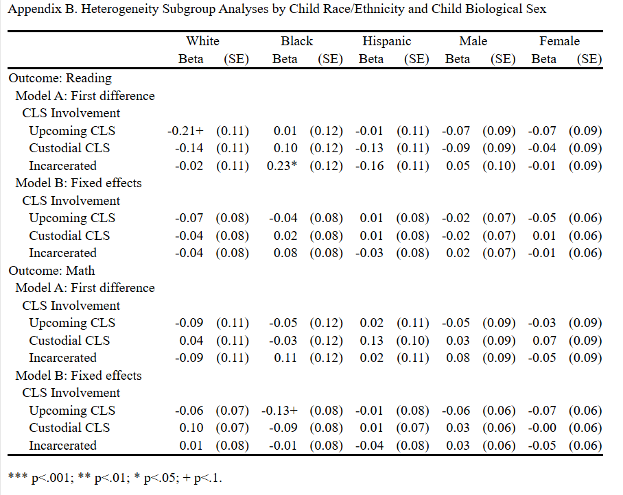
collect title "Appendix B. Heterogeneity Subgroup  Analyses by Child Race/Ethnicity and Child Biological Sex "
collect note "*** p<.001; ** p<.01; * p<.05; + p<.1."

collect style cell border_block, border(right, pattern(nil))

collect preview
Appendix B. Heterogeneity Subgroup Analyses by Child Race/Ethnicity and Child Biological Sex
----------------------------------------------------------------------------------------------
                                White         Black       Hispanic       Male        Female
                              Beta   (SE)   Beta   (SE)  Beta   (SE)  Beta   (SE)  Beta   (SE)
----------------------------------------------------------------------------------------------
Outcome: Reading
  Model A: First difference
    CLS Involvement
      Upcoming CLS          -0.21+ (0.11)   0.01 (0.12) -0.01 (0.11) -0.07 (0.09) -0.07 (0.09)
      Custodial CLS          -0.14 (0.11)   0.10 (0.12) -0.13 (0.11) -0.09 (0.09) -0.04 (0.09)
      Incarcerated           -0.02 (0.11)  0.23* (0.12) -0.16 (0.11)  0.05 (0.10) -0.01 (0.09)
  Model B: Fixed effects
    CLS Involvement
      Upcoming CLS           -0.07 (0.08)  -0.04 (0.08)  0.01 (0.08) -0.02 (0.07) -0.05 (0.06)
      Custodial CLS          -0.04 (0.08)   0.02 (0.08)  0.01 (0.08) -0.02 (0.07)  0.01 (0.06)
      Incarcerated           -0.04 (0.08)   0.08 (0.08) -0.03 (0.08)  0.02 (0.07) -0.01 (0.06)
Outcome: Math
  Model A: First difference
    CLS Involvement
      Upcoming CLS           -0.09 (0.11)  -0.05 (0.12)  0.02 (0.11) -0.05 (0.09) -0.03 (0.09)
      Custodial CLS           0.04 (0.11)  -0.03 (0.12)  0.13 (0.10)  0.03 (0.09)  0.07 (0.09)
      Incarcerated           -0.09 (0.11)   0.11 (0.12)  0.02 (0.11)  0.08 (0.09) -0.05 (0.09)
  Model B: Fixed effects
    CLS Involvement
      Upcoming CLS           -0.06 (0.07) -0.13+ (0.08) -0.01 (0.08) -0.06 (0.06) -0.07 (0.06)
      Custodial CLS           0.10 (0.07)  -0.09 (0.08)  0.01 (0.07)  0.03 (0.06) -0.00 (0.06)
      Incarcerated            0.01 (0.08)  -0.01 (0.08) -0.04 (0.08)  0.03 (0.06) -0.05 (0.06)
----------------------------------------------------------------------------------------------
*** p<.001; ** p<.01; * p<.05; + p<.1.
9.4 Comparing Coefficients
The stars in this table indicate the result of comparing each coefficient to zero, as is standard. But the original version of this table has additional notes when 1) a coefficient on a CLS level is significantly different from any other coefficient on a CLS level within the same model (e.g. if Upcoming CLS has a different effect than Custodial CLS) or 2) a coefficent is significantly different from the same coefficient in the model for a different subgroup (e.g. Upcoming CLS has a different effect for Whites than Blacks).
Question 1 is almost a contrast (see help contrast) but there isn’t a contrast operator for all possible comparisons. So instead, run a series of test commands:
test 1.cls = 2.cls
test 1.cls = 3.cls
test 2.cls = 3.cls
 ( 1)  1.cls - 2.cls = 0

       F(  1,  2057) =    1.21
            Prob > F =    0.2724

 ( 1)  1.cls - 3.cls = 0

       F(  1,  2057) =    0.18
            Prob > F =    0.6712

 ( 1)  2.cls - 3.cls = 0

       F(  1,  2057) =    0.44
            Prob > F =    0.5077
In this case, none of the coefficients are significantly different from each other.
The test commands acts on the coefficients from the last model run. To run this test on all the models, recreate the loop used to create the models (except now you can loop over diff and fe), load the results of each model, and then run the tests.
foreach var in race sex {
    levelsof `var', local(levels)
    foreach level of local levels {
        foreach outcome in reading math {
            foreach method in diff fe {
                est restore  `var'_`level'_`outcome'_`method'
                quietly: test 1.cls = 2.cls
                quietly: test 1.cls = 3.cls
                quietly: test 2.cls = 3.cls
            }
        }
    }
}
0 1 2
(results race_0_reading_diff are active now)
(results race_0_reading_fe are active now)
(results race_0_math_diff are active now)
(results race_0_math_fe are active now)
(results race_1_reading_diff are active now)
(results race_1_reading_fe are active now)
(results race_1_math_diff are active now)
(results race_1_math_fe are active now)
(results race_2_reading_diff are active now)
(results race_2_reading_fe are active now)
(results race_2_math_diff are active now)
(results race_2_math_fe are active now)
0 1
(results sex_0_reading_diff are active now)
(results sex_0_reading_fe are active now)
(results sex_0_math_diff are active now)
(results sex_0_math_fe are active now)
(results sex_1_reading_diff are active now)
(results sex_1_reading_fe are active now)
(results sex_1_math_diff are active now)
(results sex_1_math_fe are active now)I omitted the actual test results because they’re long, but you could easily scan them, identify any significant differences, and mark them in the table as you see fit.
To answer the question “Does the effect of CLS vary by race or sex?”, running separate regressions on race and sex groups and then comparing coefficients is not the right approach. (There are ways of doing it, but they’re controversial. Look up the sureg command if you ever really need to.) Instead, run a single model on the entire sample and add interaction terms between CLS and race and CLS and sex. Then the p-value on the appropriate interaction term immediately answers your question.
For example:
xtreg reading cls##(race sex), fenote: 1.race omitted because of collinearity.
note: 2.race omitted because of collinearity.
note: 1.sex omitted because of collinearity.
Fixed-effects (within) regression Number of obs = 5,000
Group variable: i Number of groups = 1,000
R-squared: Obs per group:
Within = 0.0010 min = 5
Between = 0.0002 avg = 5.0
Overall = 0.0006 max = 5
F(12, 3988) = 0.33
corr(u_i, Xb) = -0.0294 Prob > F = 0.9843
------------------------------------------------------------------------------
reading | Coefficient Std. err. t P>|t| [95% conf. interval]
-------------+----------------------------------------------------------------
cls |
-.0564579 .087205 -0.65 0.517 -.2274284 .1145126
Custodial.. | -.052055 .0880967 -0.59 0.555 -.2247737 .1206638
Incarcera~d | -.0257014 .0916166 -0.28 0.779 -.2053212 .1539183
|
race |
Black | 0 (omitted)
Hispanic | 0 (omitted)
|
sex |
Female | 0 (omitted)
|
cls#race |
Upcoming .. #|
Black | .0353462 .1119407 0.32 0.752 -.1841202 .2548125
Upcoming .. #|
Hispanic | .081172 .1104579 0.73 0.462 -.1353873 .2977313
Custodial.. #|
Black | .0533621 .1128157 0.47 0.636 -.1678199 .274544
Custodial.. #|
Hispanic | .0475723 .1091663 0.44 0.663 -.1664547 .2615994
Incarcera~d #|
Black | .1182895 .1138002 1.04 0.299 -.1048225 .3414016
Incarcera~d #|
Hispanic | .0094742 .1138465 0.08 0.934 -.2137286 .232677
|
cls#sex |
Upcoming .. #|
Female | -.0316497 .0912753 -0.35 0.729 -.2106004 .1473009
Custodial.. #|
Female | .0249265 .0910721 0.27 0.784 -.1536257 .2034787
Incarcera~d #|
Female | -.031668 .0932575 -0.34 0.734 -.2145047 .1511688
|
_cons | .0227928 .0320499 0.71 0.477 -.040043 .0856286
-------------+----------------------------------------------------------------
sigma_u | .44356047
sigma_e | 1.0161368
rho | .16004972 (fraction of variance due to u_i)
------------------------------------------------------------------------------
F test that all u_i=0: F(999, 3988) = 0.95 Prob > F = 0.8512In this case, we do not find a significant difference in the effect of any level of CLS between race or sex groups.