clear all
use https://sscc.wisc.edu/sscc/pubs/real_world_tables/table1a.dta1 Table 1 with Two Columns
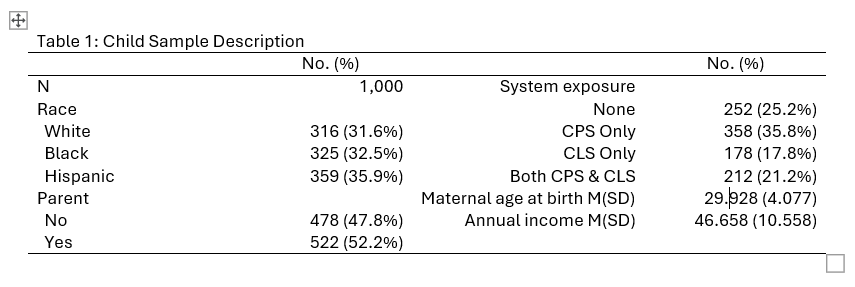
We’ll start with something that’s easy…except for the part that’s impossible.
This is a classic table of descriptive statistics, usually “Table 1” in your paper. Note that it contains both categorical variables (also known as factor variables) and quantitative variables. For the categorical variables, it gives frequencies and percentages for each category, or level. For the continuous variable it gives the mean and standard deviation, as indicated by M(SD) in the label. All that is very easy to do using the dtable command, and we’ll use this table as our introduction to dtable.
The part that’s impossible is putting the content in two columns just so it takes up less space, not because the columns have any logical meaning. This is based on a much longer table, and the goal in the original was to make everything fit on one page. Actually, putting the content in two columns is easy. What’s impossible, or at least not worth the effort, is making rows mean different things in different columns. We’ll talk about options once we’ve got the basics set up.
1.1 Setting Up
Load the data with:
Take a moment to look it over and identify the variable names.
1.2 Introducing dtable
The dtable command makes simple tables of descriptive statistics very easily. Just give it a varlist containing the variables you want to include. Put i. in front of factor variables just like when running regressions:
dtable i.race i.exposure i.parent age income
-------------------------------------------
                                Summary
-------------------------------------------
N                                     1,000
Race
  White                         316 (31.6%)
  Black                         325 (32.5%)
  Hispanic                      359 (35.9%)
System exposure
  None                          276 (27.6%)
  CPS Only                      290 (29.0%)
  CLS Only                      196 (19.6%)
  Both CPS & CLS                238 (23.8%)
Parent
  No                            478 (47.8%)
  Yes                           522 (52.2%)
Maternal age at birth M(SD)  29.928 (4.077)
Annual income M(SD)         46.658 (10.558)
-------------------------------------------
This is already a fairly nice table. The data set came with both variable and value labels already set, so dtable used them automatically. (In other examples we’ll set the labels to be used in the table ourselves.)
But dtable didn’t just make the table you see here. It also created a collection that you can further refine. To see the basic structure, run collect layout:
collect layout
Collection: DTable
      Rows: var
   Columns: result
   Table 1: 15 x 1

-------------------------------------------
                                Summary
-------------------------------------------
N                                     1,000
Race
  White                         316 (31.6%)
  Black                         325 (32.5%)
  Hispanic                      359 (35.9%)
System exposure
  None                          276 (27.6%)
  CPS Only                      290 (29.0%)
  CLS Only                      196 (19.6%)
  Both CPS & CLS                238 (23.8%)
Parent
  No                            478 (47.8%)
  Yes                           522 (52.2%)
Maternal age at birth M(SD)  29.928 (4.077)
Annual income M(SD)         46.658 (10.558)
-------------------------------------------
Rows: var tells you there’s one row for each level of a dimension called var. You can see the levels of var with:
collect levelsof var
Collection: DTable
 Dimension: var
    Levels: _N _hide 0.race 1.race 2.race 0.exposure 1.exposure 2.exposure
            3.exposure 0.parent 1.parent age income
This is fairly straightforward, other than _hide (which we don’t need and won’t discuss).
Columns: result tells you there’s one column for each level of a dimension called result. You can see the levels of result with:
collect levelsof result
Collection: DTable
 Dimension: result
    Levels: _dtable_stats _dtable_test frequency fvfrequency fvpercent mean
            percent proportion rawpercent rawproportion sd sumw
That’s a lot of levels, many more than we have in our table. That’s because only one of them is shown by default, _dtable_stats. This is a special level created by dtable to contain whatever result is appropriate for each row. Compare with:
collect layout (var) (result[fvfrequency fvpercent mean sd])
Collection: DTable
      Rows: var
   Columns: result[fvfrequency fvpercent mean sd]
   Table 1: 14 x 4

-------------------------------------------------------------------------------------------------------
                            Factor-variable frequency Factor-variable percent  Mean  Standard deviation
-------------------------------------------------------------------------------------------------------
Race
  White                                           316                 (31.6%)
  Black                                           325                 (32.5%)
  Hispanic                                        359                 (35.9%)
System exposure
  None                                            276                 (27.6%)
  CPS Only                                        290                 (29.0%)
  CLS Only                                        196                 (19.6%)
  Both CPS & CLS                                  238                 (23.8%)
Parent
  No                                              478                 (47.8%)
  Yes                                             522                 (52.2%)
Maternal age at birth M(SD)                                                   29.928            (4.077)
Annual income M(SD)                                                           46.658           (10.558)
-------------------------------------------------------------------------------------------------------
This gives all the same numbers, but each result is in its own column. The purpose of _dtable_stats is to combine them into one column:
collect layout (var) (result[_dtable_stats])
Collection: DTable
      Rows: var
   Columns: result[_dtable_stats]
   Table 1: 15 x 1

-------------------------------------------
                                Summary
-------------------------------------------
N                                     1,000
Race
  White                         316 (31.6%)
  Black                         325 (32.5%)
  Hispanic                      359 (35.9%)
System exposure
  None                          276 (27.6%)
  CPS Only                      290 (29.0%)
  CLS Only                      196 (19.6%)
  Both CPS & CLS                238 (23.8%)
Parent
  No                            478 (47.8%)
  Yes                           522 (52.2%)
Maternal age at birth M(SD)  29.928 (4.077)
Annual income M(SD)         46.658 (10.558)
-------------------------------------------
The column header Summary is intended to cover describe factor and quantitative variables, but our source table instead labels it for just the factor variables and puts M(SD) in the row labels for the quantitative variables to indicate they are exceptions. You can change the header of the column by applying a new label to the dtable_stats level of result:
collect label levels result _dtable_stats "No. (%)", modifyAdd a title to the table with collect title:
collect title "Table 1: Child Sample Description"
collect preview
Table 1: Child Sample Description
-------------------------------------------
                                No. (%)
-------------------------------------------
N                                     1,000
Race
  White                         316 (31.6%)
  Black                         325 (32.5%)
  Hispanic                      359 (35.9%)
System exposure
  None                          276 (27.6%)
  CPS Only                      290 (29.0%)
  CLS Only                      196 (19.6%)
  Both CPS & CLS                238 (23.8%)
Parent
  No                            478 (47.8%)
  Yes                           522 (52.2%)
Maternal age at birth M(SD)  29.928 (4.077)
Annual income M(SD)         46.658 (10.558)
-------------------------------------------
1.3 Splitting the “Columns”
This table is quite usable as-is. But if you really want to break it up into two columns, you need to designate which elements will be part of which columns. To do that, you’ll create a new dimension called col with the levels 1 and 2.
You can add new tags to elements of the collection with collect addtag. It is followed by the tag to add. Then the fortags options specifies which elements the new tag is to be applied to.
Recall that the var dimension, which controls the rows, has a level _N (number of observations) and a level for each category of the categorical variables as well as one for each quantitative variable. Apply the tag col[1] to _N and all the levels of race and parent with:
collect addtag col[1], fortags(var[_N i.race i.parent])(12 items changed in collection DTable)Now apply the tag col[2] to all the levels of exposure as well as age and income with:
collect addtag col[2], fortags(var[i.exposure age income])(12 items changed in collection DTable)You can then use col to define supercolumns within the table with:
collect layout (var) (col#result[_dtable_stats])
Collection: DTable
      Rows: var
   Columns: col#result[_dtable_stats]
   Table 1: 15 x 2

Table 1: Child Sample Description
-------------------------------------------------------
                                 1             2
                              No. (%)       No. (%)
-------------------------------------------------------
N                                 1,000
Race
  White                     316 (31.6%)
  Black                     325 (32.5%)
  Hispanic                  359 (35.9%)
System exposure
  None                                      276 (27.6%)
  CPS Only                                  290 (29.0%)
  CLS Only                                  196 (19.6%)
  Both CPS & CLS                            238 (23.8%)
Parent
  No                        478 (47.8%)
  Yes                       522 (52.2%)
Maternal age at birth M(SD)              29.928 (4.077)
Annual income M(SD)                     46.658 (10.558)
-------------------------------------------------------
Well, that gave you two columns, but it didn’t save you any space. As mentioned earlier, the problem is that a row can only mean one thing. The first row cannot be N in column 1 and System exposure in column 2. Some options:
- Create a new dimension to control the rows, along with four new columns: label of the first column variable, result for the first column variable, label for the second column variable, result for the second column variable. This should be doable, but messy.
- Use
collect export’sdofile()option to have it create a do file containing all theputdocxcommands needed to create the table, then edit that do file. That will give you total control of the table that’s created, but is even messier. - Export the table to a
docxfile, open it in Word, and simply move half the results into a second column. This is by far the easiest solution, but it is not fully reproducible: if you ever have to change the table, you’ll need to repeat those steps in Word again.
I used the third option to create the example at the top of this page. This highlights the fact that you can spend an awful lot of time trying to do things that are hard in Stata but very simple in Word. When to spend that time is a judgment call, and depends on the details of your project. If you need to make 100 similar tables, or need to create a new table every month as new data arrives, you want a fully automated solution. But for a typical paper, spending a little time polishing up the look of a table in Word is probably acceptable.
You can make moving half the results easier by making a separate table for each column:
collect layout (var) (result[_dtable_stats]) (col)
Collection: DTable
      Rows: var
   Columns: result[_dtable_stats]
    Tables: col
   Table 1: 8 x 1
   Table 2: 7 x 1

Table 1: Child Sample Description
----------------------
             No. (%)
----------------------
N                1,000
Race
  White    316 (31.6%)
  Black    325 (32.5%)
  Hispanic 359 (35.9%)
Parent
  No       478 (47.8%)
  Yes      522 (52.2%)
----------------------

Table 1: Child Sample Description
-------------------------------------------
                                No. (%)
-------------------------------------------
System exposure
  None                          276 (27.6%)
  CPS Only                      290 (29.0%)
  CLS Only                      196 (19.6%)
  Both CPS & CLS                238 (23.8%)
Maternal age at birth M(SD)  29.928 (4.077)
Annual income M(SD)         46.658 (10.558)
-------------------------------------------
If you export this to Word (collect export table1_a.docx, replace) you can click on the first table, add a column to it, and then paste the second table into the new column. That’s how I created the example at the beginning of the chapter.