clear all
use https://sscc.wisc.edu/sscc/pubs/real_world_tables/table1b2 Table 1 with Hierarchical Data
This is another Table 1, but the complication this time is that it’s for hierarchical data. The data set consists of children who can have multiple placements into foster homes, and we want summary statistics both by child and by placement.
2.1 Setting up
Load the data with:
Take a moment to look it over and identify the variable names.
2.2 tag and by
The egen function tag() takes an identifier variable as its argument, and then creates a new variable which is 1 for the first observation for that identifier, and zero for all the others. (Note that this has nothing to do with the tags used by collect.)
This data set has a variable id that identifies all the placements for a given child, so create a tag for each child with:
egen child = tag(id)The classic use of a tag like this is in an if condition. For example, compare:
tab sex
        Sex |      Freq.     Percent        Cum.
------------+-----------------------------------
       Male |      1,717       58.88       58.88
     Female |      1,199       41.12      100.00
------------+-----------------------------------
      Total |      2,916      100.00
tab sex if child
        Sex |      Freq.     Percent        Cum.
------------+-----------------------------------
       Male |        516       51.60       51.60
     Female |        484       48.40      100.00
------------+-----------------------------------
      Total |      1,000      100.00
The first table gives the frequencies of sex for all the placements. The second gives the frequencies of sex for all the children. The percentages are different because in this (made up) data set boys tend to have more placements.
Now create a table of descriptive statistics, adding the by(child) option:
dtable i.race i.sex, by(child)
-----------------------------------------------------
                             tag(id)
                 0             1            Total
-----------------------------------------------------
N          1,916 (65.7%) 1,000 (34.3%) 2,916 (100.0%)
Race
  White      675 (35.2%)   340 (34.0%)  1,015 (34.8%)
  Black      612 (31.9%)   329 (32.9%)    941 (32.3%)
  Hispanic   629 (32.8%)   331 (33.1%)    960 (32.9%)
Sex
  Male     1,201 (62.7%)   516 (51.6%)  1,717 (58.9%)
  Female     715 (37.3%)   484 (48.4%)  1,199 (41.1%)
-----------------------------------------------------
This gives three sets of descriptive statistics: one for the observations where child is zero, one for the observations where child is one, and one (Total) for all observations.
The group where child is zero contains all the observations other than the first observation for each child. You’re not interested in the descriptive statistics for this group.
The group where child is one contains one observation per child and thus gives child-level descriptive statistics. (Note how it matches the second set of frequencies calculated earlier.) You want these descriptive statistics.
The descriptive statistics for all observations gives placement-level descriptive statistics. You want these descriptive statistics too.
Take a look at the layout of this collection:
collect layout
Collection: DTable
      Rows: var
   Columns: child#result
   Table 1: 8 x 3

-----------------------------------------------------
                             tag(id)
                 0             1            Total
-----------------------------------------------------
N          1,916 (65.7%) 1,000 (34.3%) 2,916 (100.0%)
Race
  White      675 (35.2%)   340 (34.0%)  1,015 (34.8%)
  Black      612 (31.9%)   329 (32.9%)    941 (32.3%)
  Hispanic   629 (32.8%)   331 (33.1%)    960 (32.9%)
Sex
  Male     1,201 (62.7%)   516 (51.6%)  1,717 (58.9%)
  Female     715 (37.3%)   484 (48.4%)  1,199 (41.1%)
-----------------------------------------------------
You have one column per level of child per level of result. Get a list of the levels of child with:
collect levelsof child
Collection: DTable
 Dimension: child
    Levels: 0 1 .m
.m is the Total column. You’re interested in that and the 1 column, so specify that only those levels should be included. Also specify that the number of observations (_N) should come at the end rather than the beginning by listing the levels of var in the order you want:
collect layout (var[i.race i.sex _N]) (child[1 .m]#result)
Collection: DTable
      Rows: var[i.race i.sex _N]
   Columns: child[1 .m]#result
   Table 1: 8 x 2

---------------------------------------
                      tag(id)
                 1            Total
---------------------------------------
Race
  White      340 (34.0%)  1,015 (34.8%)
  Black      329 (32.9%)    941 (32.3%)
  Hispanic   331 (33.1%)    960 (32.9%)
Sex
  Male       516 (51.6%)  1,717 (58.9%)
  Female     484 (48.4%)  1,199 (41.1%)
N          1,000 (34.3%) 2,916 (100.0%)
---------------------------------------
Next change the labels for the child dimension:
collect label levels child 1 "Child" .m "Placement", modifyThe label tag(id) is the variable label egen created for the child variable. dtable used it as the title for the child header. You don’t really need anything there, so hide that title:
collect style header child, title(hide) Finally, change the label for _N from N to Sample Size. (This is purely a matter of taste.)
collect label levels var _N "Sample Size", modify
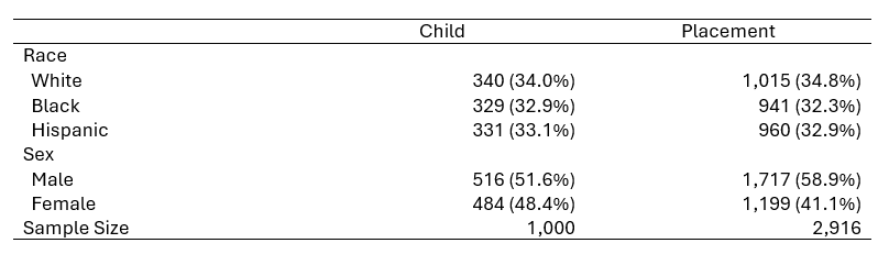
collect preview
----------------------------------------
                Child        Placement
----------------------------------------
Race
  White       340 (34.0%)  1,015 (34.8%)
  Black       329 (32.9%)    941 (32.3%)
  Hispanic    331 (33.1%)    960 (32.9%)
Sex
  Male        516 (51.6%)  1,717 (58.9%)
  Female      484 (48.4%)  1,199 (41.1%)
Sample Size 1,000 (34.3%) 2,916 (100.0%)
----------------------------------------
2.3 collect unget
Better, but the percentages on Sample Size don’t make much sense.
As of Stata 19 you can remove items from the result dimension with collect unget. Just specify the result to be removed and for which tags:
collect unget percent, fortags(var[_N])
collect preview
(3 items removed from collection DTable)
-------------------------------------
Child Placement
-------------------------------------
Race
White 340 (34.0%) 1,015 (34.8%)
Black 329 (32.9%) 941 (32.3%)
Hispanic 331 (33.1%) 960 (32.9%)
Sex
Male 516 (51.6%) 1,717 (58.9%)
Female 484 (48.4%) 1,199 (41.1%)
Sample Size 1,000 2,916
-------------------------------------