clear all
use https://sscc.wisc.edu/sscc/pubs/real_world_tables/reg14 Multinomial Logit
Shifting now to tables of regression results, our first challenge is a multinomial regression model, where each outcome has its own set of coefficients. Our goal is to put them in separate columns. We also want relative risk ratios and confidence intervals, on one row, rather than coefficients and standard errors.
4.1 Setting Up
Load the data and take a moment to look it over and identify the variables.
4.2 Run the Model and Collect the Results
Run the regression model, including the rrr option to report relative risk ratios, and collect the results:
collect: mlogit involvement i.exposure i.race, rrr base(0)
Iteration 0:  Log likelihood = -1373.9734
Iteration 1:  Log likelihood = -1326.0187
Iteration 2:  Log likelihood = -1325.2431
Iteration 3:  Log likelihood = -1325.2429
Iteration 4:  Log likelihood = -1325.2429

Multinomial logistic regression                         Number of obs =  1,000
                                                        LR chi2(15)   =  97.46
                                                        Prob > chi2   = 0.0000
Log likelihood = -1325.2429                             Pseudo R2     = 0.0355

------------------------------------------------------------------------------
 involvement |        RRR   Std. err.      z    P>|z|     [95% conf. interval]
-------------+----------------------------------------------------------------
None         |  (base outcome)
-------------+----------------------------------------------------------------
CPS_Only     |
    exposure |
   CPS Only  |   2.520022   .6523992     3.57   0.000      1.51719    4.185707
   CLS Only  |   1.563043   .4670294     1.49   0.135     .8702346    2.807409
Both CPS ..  |   1.258737   .3508603     0.83   0.409     .7289055    2.173697
             |
        race |
      Black  |   1.173601   .2837658     0.66   0.508     .7306474    1.885094
   Hispanic  |   .9474532    .221673    -0.23   0.818     .5989693    1.498687
             |
       _cons |   .6896629   .1616981    -1.58   0.113     .4355765    1.091966
-------------+----------------------------------------------------------------
CLS_Only     |
    exposure |
   CPS Only  |   .8276127   .2105479    -0.74   0.457     .5026645    1.362624
   CLS Only  |   2.539109   .6393221     3.70   0.000     1.550092    4.159157
Both CPS ..  |    .725354   .1884331    -1.24   0.216     .4359374    1.206913
             |
        race |
      Black  |   1.155772   .2583481     0.65   0.517     .7457687    1.791183
   Hispanic  |   .6523108   .1456247    -1.91   0.056     .4211421     1.01037
             |
       _cons |   1.416345   .2906654     1.70   0.090     .9472914    2.117651
-------------+----------------------------------------------------------------
Both_CPS__~S |
    exposure |
   CPS Only  |   .9414855   .2508099    -0.23   0.821     .5585413    1.586982
   CLS Only  |   1.702195   .4650387     1.95   0.052     .9964641     2.90775
Both CPS ..  |   1.685971   .4183011     2.11   0.035     1.036719    2.741821
             |
        race |
      Black  |   1.434602   .3397596     1.52   0.128     .9018611    2.282039
   Hispanic  |   1.218457   .2747452     0.88   0.381     .7832058     1.89559
             |
       _cons |   .8273178   .1839026    -0.85   0.394     .5351317     1.27904
------------------------------------------------------------------------------
Note: _cons estimates baseline relative risk for each outcome.
4.3 Structure the Table
To see what’s in the collection, run collect dims:
collect dims
Collection dimensions
Collection: default
-----------------------------------------
                   Dimension   No. levels
-----------------------------------------
Layout, style, header, label
                      cmdset   1
                       coleq   4
                     colname   13
           colname_remainder   1
                    exposure   4
               program_class   1
                        race   3
                      result   48
                 result_type   3
                     rowname   1

Style only
                border_block   4
                   cell_type   4
-----------------------------------------
As usual, colname contains the predictors. It will be the rows of the table, but we’ll select only i.exposure and i.race.
collect levelsof colname
Collection: default
 Dimension: colname
    Levels: 0.exposure 1.exposure 2.exposure 3.exposure 0.race 1.race 2.race
            c1 c2 c3 c4 _cons o._cons
result contains the various available results from the model.
collect levelsof result
Collection: default
 Dimension: result
    Levels: N N_cd _r_b _r_ci _r_df _r_lb _r_p _r_se _r_ub _r_z _r_z_abs
            baselab baseout chi2 chi2type cmd cmdline converged depvar
            deriv_useminbound df_m eqnames ibaseout ic k k_dv k_eq k_eq_base
            k_eq_model k_out ll ll_0 marginsdefault marginsnotok ml_method
            opt out p predict properties r2_p rank rc technique title user
            vce which
result[_r_b] contains the coefficients as reported by the regression command, so in this case they are actually the relative risk ratios. result[_r_ci] contains the confidence intervals. We want the risk ratios and confidence intervals on the same row in two columns, so result[_r_b _r_ci] will be part of the column specification.
What about the four outcomes? They are found in coleq:
collect levelsof coleq
Collection: default
 Dimension: coleq
    Levels: None CPS_Only CLS_Only Both_CPS___CLS
The names of the levels are based on the value labels for the outcome variable, involvement. But they contain characters that can’t be used in collection levels, so collect had to adapt them.
The layout you need is:
collect layout (colname[i.exposure i.race]) (coleq[CPS_Only CLS_Only Both_CPS___CLS]#result[_r_b _r_ci])
Collection: default
      Rows: colname[i.exposure i.race]
   Columns: coleq[CPS_Only CLS_Only Both_CPS___CLS]#result[_r_b _r_ci]
   Table 1: 7 x 6

----------------------------------------------------------------------------------------------------------------
               |    CPS_Only           CPS_Only    CLS_Only           CLS_Only Both_CPS___CLS     Both_CPS___CLS
               | Coefficient       95% CI       Coefficient       95% CI          Coefficient       95% CI
---------------+------------------------------------------------------------------------------------------------
None           |           1                              1                                 1
CPS Only       |    2.520022  1.51719  4.185707    .8276127 .5026645  1.362624       .9414855 .5585413  1.586982
CLS Only       |    1.563043 .8702346  2.807409    2.539109 1.550092  4.159157       1.702195 .9964641   2.90775
Both CPS & CLS |    1.258737 .7289055  2.173697     .725354 .4359374  1.206913       1.685971 1.036719  2.741821
White          |           1                              1                                 1
Black          |    1.173601 .7306474  1.885094    1.155772 .7457687  1.791183       1.434602 .9018611  2.282039
Hispanic       |    .9474532 .5989693  1.498687    .6523108 .4211421   1.01037       1.218457 .7832058   1.89559
----------------------------------------------------------------------------------------------------------------
This omits the “model” for the base outcome (all ones) as well as specifying which results to include.
4.4 Clean Up
This is the structure we want, but the are a bunch of settings that need tweaking to give it a satisfactory appearance. Styles are collections of such settings, and can save you some work if you like what they do. Stata comes with some styles predefined, and you can create your own if you find yourself using the same settings repeatedly. In this case, the style table-reg1 will help with the columns headers, so apply it with collect style use:
collect style use table-reg1
collect preview
Collection: default
      Rows: colname[i.exposure i.race]
   Columns: coleq[CPS_Only CLS_Only Both_CPS___CLS]#result[_r_b _r_ci]
   Table 1: 7 x 6

------------------------------------------------------------------------------------------------------------------------
               |              CPS_Only                           CLS_Only                        Both_CPS___CLS
               |  Coefficient         95% CI         Coefficient         95% CI         Coefficient         95% CI
---------------+--------------------------------------------------------------------------------------------------------
None           |            1                                  1                                  1
CPS Only       |     2.520022    1.51719  4.185707      .8276127   .5026645  1.362624      .9414855   .5585413  1.586982
CLS Only       |     1.563043   .8702346  2.807409      2.539109   1.550092  4.159157      1.702195   .9964641   2.90775
Both CPS & CLS |     1.258737   .7289055  2.173697       .725354   .4359374  1.206913      1.685971   1.036719  2.741821
White          |            1                                  1                                  1
Black          |     1.173601   .7306474  1.885094      1.155772   .7457687  1.791183      1.434602   .9018611  2.282039
Hispanic       |     .9474532   .5989693  1.498687      .6523108   .4211421   1.01037      1.218457   .7832058   1.89559
------------------------------------------------------------------------------------------------------------------------
The list of variables on the left is missing the names of the factor variables. Turn them on and stack them:
collect style header exposure race, title(label)
collect style row stack, nobinder
collect preview
--------------------------------------------------------------------------------------------------------------------------
                 |              CPS_Only                           CLS_Only                        Both_CPS___CLS
                 |  Coefficient         95% CI         Coefficient         95% CI         Coefficient         95% CI
-----------------+--------------------------------------------------------------------------------------------------------
System Exposure  |
  None           |            1                                  1                                  1
  CPS Only       |     2.520022    1.51719  4.185707      .8276127   .5026645  1.362624      .9414855   .5585413  1.586982
  CLS Only       |     1.563043   .8702346  2.807409      2.539109   1.550092  4.159157      1.702195   .9964641   2.90775
  Both CPS & CLS |     1.258737   .7289055  2.173697       .725354   .4359374  1.206913      1.685971   1.036719  2.741821
Race             |
  White          |            1                                  1                                  1
  Black          |     1.173601   .7306474  1.885094      1.155772   .7457687  1.791183      1.434602   .9018611  2.282039
  Hispanic       |     .9474532   .5989693  1.498687      .6523108   .4211421   1.01037      1.218457   .7832058   1.89559
--------------------------------------------------------------------------------------------------------------------------
You don’t need the base categories:`
collect style showbase off
collect preview
--------------------------------------------------------------------------------------------------------------------------
                 |              CPS_Only                           CLS_Only                        Both_CPS___CLS
                 |  Coefficient         95% CI         Coefficient         95% CI         Coefficient         95% CI
-----------------+--------------------------------------------------------------------------------------------------------
System Exposure  |
  CPS Only       |     2.520022    1.51719  4.185707      .8276127   .5026645  1.362624      .9414855   .5585413  1.586982
  CLS Only       |     1.563043   .8702346  2.807409      2.539109   1.550092  4.159157      1.702195   .9964641   2.90775
  Both CPS & CLS |     1.258737   .7289055  2.173697       .725354   .4359374  1.206913      1.685971   1.036719  2.741821
Race             |
  Black          |     1.173601   .7306474  1.885094      1.155772   .7457687  1.791183      1.434602   .9018611  2.282039
  Hispanic       |     .9474532   .5989693  1.498687      .6523108   .4211421   1.01037      1.218457   .7832058   1.89559
--------------------------------------------------------------------------------------------------------------------------
You don’t need this many digits: three will be plenty, and you can do that with nformat(). Normally the maximum amount of digits in the format doesn’t matter much, but in this case Stata will reserve that many spaces for the upper bound of the confidence interval. So instead of using %8.3f, use %5.3f so there are no extra spaces.
You also want to put the confidence intervals in square brackets, which can be done with sformat(). Recall that in defining an sformat, the value itself is %s. To put a dash between the upper and lower bounds of the confidence interval, use cidelimiter().
collect style cell result, nformat(%5.3f)
collect style cell result[_r_ci], sformat("[%s]") cidelimiter("-")
collect preview
-----------------------------------------------------------------------------------------------------------
                 |            CPS_Only                      CLS_Only                   Both_CPS___CLS
                 |  Coefficient       95% CI      Coefficient       95% CI      Coefficient       95% CI
-----------------+-----------------------------------------------------------------------------------------
System Exposure  |
  CPS Only       |        2.520   [1.517-4.186]         0.828   [0.503-1.363]         0.941   [0.559-1.587]
  CLS Only       |        1.563   [0.870-2.807]         2.539   [1.550-4.159]         1.702   [0.996-2.908]
  Both CPS & CLS |        1.259   [0.729-2.174]         0.725   [0.436-1.207]         1.686   [1.037-2.742]
Race             |
  Black          |        1.174   [0.731-1.885]         1.156   [0.746-1.791]         1.435   [0.902-2.282]
  Hispanic       |        0.947   [0.599-1.499]         0.652   [0.421-1.010]         1.218   [0.783-1.896]
-----------------------------------------------------------------------------------------------------------
Next let’s improve the column headers. Add an explanatory title above the outcomes by adding a label to the coleq dimension and then show it:
collect label dim coleq "System involvement (ref: none)", modify
collect style header coleq, title(label)
The label for the levels of coleq also need improvement. Add the number of observations for each outcome like in the previous chapter:
count if involvement==1
local n1 = r(N)
count if involvement==2
local n2 = r(N)
count if involvement==3
local n3 = r(N)
collect label levels coleq CPS_Only "CPS Only (N=`n1')" CLS_Only "CLS_Only (N=`n2')" Both_CPS___CLS "Both CPS & CLS (N=`n3')", modify
225
309
261Finally, relabel the relevant levels of result to say you are using relative risk ratios (RRR) rather than coefficients.
collect label levels result _r_b "RRR" _r_ci "95% CI", modify

collect preview
--------------------------------------------------------------------------------------------
                 |                       System involvement (ref: none)
                 |     CPS Only (N=225)        CLS_Only (N=309)      Both CPS & CLS (N=261)
                 |    RRR       95% CI        RRR       95% CI          RRR       95% CI
-----------------+--------------------------------------------------------------------------
System Exposure  |
  CPS Only       |  2.520   [1.517-4.186]   0.828   [0.503-1.363]     0.941    [0.559-1.587]
  CLS Only       |  1.563   [0.870-2.807]   2.539   [1.550-4.159]     1.702    [0.996-2.908]
  Both CPS & CLS |  1.259   [0.729-2.174]   0.725   [0.436-1.207]     1.686    [1.037-2.742]
Race             |
  Black          |  1.174   [0.731-1.885]   1.156   [0.746-1.791]     1.435    [0.902-2.282]
  Hispanic       |  0.947   [0.599-1.499]   0.652   [0.421-1.010]     1.218    [0.783-1.896]
--------------------------------------------------------------------------------------------
Add stars for significance, a note explaining them, and a title for the table:
collect style cell result[_r_b], sformat("%s ")
collect stars _r_p .001 "***" .01 "** " .05 "* " .1 "+ " 1 " ", attach(_r_b)
collect note "*** p<.001; ** p<.01; * p<.05; + p<.1."
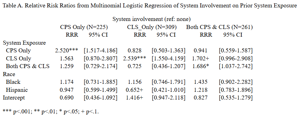
collect title "Table A. Relative Risk Ratios from Multinomial Logistic Regression of System Involvement on Prior System Exposure"Last of all, remove all the borders. This is done by styling the border_block cells. In the border() option, you can name a specific border or leave it blank to control all borders. To remove a border set its pattern to nil:
collect style cell border_block, border(, pattern(nil))
collect preview
Table A. Relative Risk Ratios from Multinomial Logistic Regression of System Involvement on Prior System Exposure
                                           System involvement (ref: none)
                       CPS Only (N=225)            CLS_Only (N=309)        Both CPS & CLS (N=261)
                        RRR       95% CI            RRR       95% CI           RRR       95% CI
System Exposure
  CPS Only        2.520***    [1.517-4.186]      0.828    [0.503-1.363]     0.941    [0.559-1.587]
  CLS Only           1.563    [0.870-2.807]   2.539***    [1.550-4.159]    1.702+    [0.996-2.908]
  Both CPS & CLS     1.259    [0.729-2.174]      0.725    [0.436-1.207]    1.686*    [1.037-2.742]
Race
  Black              1.174    [0.731-1.885]      1.156    [0.746-1.791]     1.435    [0.902-2.282]
  Hispanic           0.947    [0.599-1.499]     0.652+    [0.421-1.010]     1.218    [0.783-1.896]
*** p<.001; ** p<.01; * p<.05; + p<.1.