clear all
use https://sscc.wisc.edu/sscc/pubs/real_world_tables/reg25 Multiple Models
Now we’ll consider a table containing results from a family of related regression models. The data consists of math scores for students over multiple years, and the research question is what effect their parents’ involvement in the criminal legal system has on those scores. The models will deal with the panel structure of the data in different ways:
- Ignore it and include no controls
- Ignore it but include controls
- Regress the first differences of the math scores on first differences of the continuous variables (and ordinary values of the categorical variables)
- Include student-level fixed effects
All but the last are problematic, to say the least.
5.1 Setting Up
Load the data with:
Take a moment to look it over and identify the variable names. Note that it has already been xtset:
xtset
Panel variable: id (strongly balanced)
 Time variable: grade, 3 to 8
         Delta: 1 unit
5.2 Introducing etable
etable is a tool for quickly and easily creating tables of estimation results, just like dtable is for descriptive statistics. It’s especially useful for tables like this where you want one column per model: just store the results of each model with estimates store and then give them all to etable. The downside of etable is that the collections it creates are a little more complicated than what you’d create on your own, and sometimes customizing them is difficult.
Begin by running the four models and storing their results. The first two are straightforward:
reg math i.involvement
est sto m1
      Source |       SS           df       MS      Number of obs   =     6,000
-------------+----------------------------------   F(3, 5996)      =    115.53
       Model |  181896.455         3  60632.1516   Prob > F        =    0.0000
    Residual |  3146819.51     5,996  524.819798   R-squared       =    0.0546
-------------+----------------------------------   Adj R-squared   =    0.0542
       Total |  3328715.96     5,999  554.878474   Root MSE        =    22.909

------------------------------------------------------------------------------
        math | Coefficient  Std. err.      t    P>|t|     [95% conf. interval]
-------------+----------------------------------------------------------------
 involvement |
  -4.317182   .8381054    -5.15   0.000     -5.96017   -2.674194
Noncustod..  |  -10.36844   .8338804   -12.43   0.000    -12.00314   -8.733731
Incarcera..  |  -14.31858   .8345743   -17.16   0.000    -15.95464   -12.68251
             |
       _cons |    95.2052   .5893494   161.54   0.000     94.04986    96.36053
------------------------------------------------------------------------------
reg math i.race ib1.sex i.involvement i.homeless income
est sto m2
      Source |       SS           df       MS      Number of obs   =     6,000
-------------+----------------------------------   F(8, 5991)      =    286.25
       Model |   920511.34         8  115063.918   Prob > F        =    0.0000
    Residual |  2408204.62     5,991  401.970393   R-squared       =    0.2765
-------------+----------------------------------   Adj R-squared   =    0.2756
       Total |  3328715.96     5,999  554.878474   Root MSE        =    20.049

------------------------------------------------------------------------------
        math | Coefficient  Std. err.      t    P>|t|     [95% conf. interval]
-------------+----------------------------------------------------------------
        race |
      Black  |   -.199612   .6254491    -0.32   0.750    -1.425717    1.026494
   Hispanic  |   .9282089   .6376413     1.46   0.146    -.3217976    2.178215
             |
         sex |
       Male  |   .8087496   .5192684     1.56   0.119    -.2092034    1.826703
             |
 involvement |
Upcoming ..  |  -4.853873   .7338797    -6.61   0.000    -6.292541   -3.415204
Noncustod..  |  -10.51076   .7301789   -14.39   0.000    -11.94217   -9.079342
Incarcera..  |  -14.91268   .7310017   -20.40   0.000    -16.34571   -13.47965
             |
    homeless |
   Homeless  |  -9.993068   .5178194   -19.30   0.000    -11.00818   -8.977956
      income |   .9912966   .0259119    38.26   0.000     .9404999    1.042093
       _cons |    50.4365   1.487211    33.91   0.000     47.52103    53.35197
------------------------------------------------------------------------------
The third model uses the first difference operator on the outcome and the continuous predictor income. Thus changes in math score are regressed on changes in income.
Consider taking first differences on an indicator variable, like “parent is incarcerated.” The possible values are 1 (parent became incarcerated this year), 0 (no change in incarceration status), and -1 (parent stopped being incarcerated this year). This implies that being incarcerated has no effect on the change in math scores, just entering or leaving that state. Unlikely! Unless the result is treated as a categorical variable, it further implies that entering and leaving incarceration have the same effect, just with opposite signs. So we won’t take first differences of the indicator variables in the model.
reg d.math i.race ib1.sex i.involvement i.homeless d.income
est sto m3
      Source |       SS           df       MS      Number of obs   =     5,000
-------------+----------------------------------   F(8, 4991)      =    178.10
       Model |  1207482.77         8  150935.346   Prob > F        =    0.0000
    Residual |  4229805.69     4,991  847.486614   R-squared       =    0.2221
-------------+----------------------------------   Adj R-squared   =    0.2208
       Total |  5437288.46     4,999  1087.67523   Root MSE        =    29.112

------------------------------------------------------------------------------
      D.math | Coefficient  Std. err.      t    P>|t|     [95% conf. interval]
-------------+----------------------------------------------------------------
        race |
      Black  |   .1125017   .9951498     0.11   0.910    -1.838429    2.063433
   Hispanic  |  -.5986566   1.014023    -0.59   0.555    -2.586587    1.389273
             |
         sex |
       Male  |  -.3857449   .8260016    -0.47   0.641    -2.005071    1.233581
             |
 involvement |
Upcoming ..  |  -4.679474   1.170149    -4.00   0.000     -6.97348   -2.385467
Noncustod..  |   -10.4147   1.164122    -8.95   0.000    -12.69689   -8.132511
Incarcera..  |  -14.23388   1.160735   -12.26   0.000    -16.50943   -11.95833
             |
    homeless |
   Homeless  |  -8.386708   .8237638   -10.18   0.000    -10.00165   -6.771769
             |
      income |
         D1. |   .9812488   .0289102    33.94   0.000     .9245722    1.037925
             |
       _cons |   11.91864   1.168454    10.20   0.000     9.627954    14.20932
------------------------------------------------------------------------------
Note that the outcome variable is now listed as D.math rather than math. That’s going to be important.
Finally, the fixed effects model, run using xtreg:
xtreg math i.race ib1.sex i.involvement i.homeless income, fe
est sto m4
note: 1.race omitted because of collinearity.
note: 2.race omitted because of collinearity.
note: 0.sex omitted because of collinearity.
Fixed-effects (within) regression Number of obs = 6,000
Group variable: id Number of groups = 1,000
R-squared: Obs per group:
Within = 0.2781 min = 6
Between = 0.2639 avg = 6.0
Overall = 0.2756 max = 6
F(5, 4995) = 384.81
corr(u_i, Xb) = 0.0038 Prob > F = 0.0000
------------------------------------------------------------------------------
math | Coefficient Std. err. t P>|t| [95% conf. interval]
-------------+----------------------------------------------------------------
race |
Black | 0 (omitted)
Hispanic | 0 (omitted)
|
sex |
Male | 0 (omitted)
|
involvement |
Upcoming .. | -5.014169 .8055051 -6.22 0.000 -6.593313 -3.435026
Noncustod.. | -10.86874 .7965589 -13.64 0.000 -12.43035 -9.307136
Incarcera.. | -14.4173 .7937111 -18.16 0.000 -15.97332 -12.86128
|
homeless |
Homeless | -9.859517 .5615498 -17.56 0.000 -10.9604 -8.758633
income | .9967796 .0281819 35.37 0.000 .9415307 1.052028
_cons | 50.70355 1.530615 33.13 0.000 47.70287 53.70422
-------------+----------------------------------------------------------------
sigma_u | 8.3779423
sigma_e | 19.962439
rho | .14975802 (fraction of variance due to u_i)
------------------------------------------------------------------------------
F test that all u_i=0: F(999, 4995) = 1.06 Prob > F = 0.1331Race and sex are omitted because they do not change over time and are thus collinear with the fixed effect.
Now put all four models in a table with etable. The estimates option is where you list the four sets of stored results to use. showstars adds stars for significance; showstarsnote adds a note explaining them.
etable, estimates(m1 m2 m3 m4) showstars showstarsnote
------------------------------------------------------------------------
                                math       math      D.math      math
------------------------------------------------------------------------
CLS involvement
  Upcoming CLS involvement    -4.317 **  -4.854 **             -5.014 **
                             (0.838)    (0.734)               (0.806)
  Noncustodial CLS currently -10.368 ** -10.511 **            -10.869 **
                             (0.834)    (0.730)               (0.797)
  Incarcerated currently     -14.319 ** -14.913 **            -14.417 **
                             (0.835)    (0.731)               (0.794)
Race
  Black                                  -0.200
                                        (0.625)
  Hispanic                                0.928
                                        (0.638)
Sex
  Male                                    0.809
                                        (0.519)
homeless
  Homeless                               -9.993 **             -9.860 **
                                        (0.518)               (0.562)
income                                    0.991 **              0.997 **
                                        (0.026)               (0.028)
Intercept                     95.205 **  50.437 **             50.704 **
                             (0.589)    (1.487)               (1.531)
CLS involvement
  Upcoming CLS involvement                          -4.679 **
                                                   (1.170)
  Noncustodial CLS currently                       -10.415 **
                                                   (1.164)
  Incarcerated currently                           -14.234 **
                                                   (1.161)
Race
  Black                                              0.113
                                                   (0.995)
  Hispanic                                          -0.599
                                                   (1.014)
Sex
  Male                                              -0.386
                                                   (0.826)
homeless
  Homeless                                          -8.387 **
                                                   (0.824)
D.income                                             0.981 **
                                                   (0.029)
Intercept                                           11.919 **
                                                   (1.168)
Number of observations          6000       6000       5000       6000
------------------------------------------------------------------------
** p<.01, * p<.05
5.3 Reorganize
To understand this table, take a look at its layout:
collect layout
Collection: ETable
      Rows: coleq#colname[]#result[_r_b _r_se] result[N]
   Columns: etable_depvar#stars
   Table 1: 45 x 8

------------------------------------------------------------------------
                                math       math      D.math      math
------------------------------------------------------------------------
CLS involvement
  Upcoming CLS involvement    -4.317 **  -4.854 **             -5.014 **
                             (0.838)    (0.734)               (0.806)
  Noncustodial CLS currently -10.368 ** -10.511 **            -10.869 **
                             (0.834)    (0.730)               (0.797)
  Incarcerated currently     -14.319 ** -14.913 **            -14.417 **
                             (0.835)    (0.731)               (0.794)
Race
  Black                                  -0.200
                                        (0.625)
  Hispanic                                0.928
                                        (0.638)
Sex
  Male                                    0.809
                                        (0.519)
homeless
  Homeless                               -9.993 **             -9.860 **
                                        (0.518)               (0.562)
income                                    0.991 **              0.997 **
                                        (0.026)               (0.028)
Intercept                     95.205 **  50.437 **             50.704 **
                             (0.589)    (1.487)               (1.531)
CLS involvement
  Upcoming CLS involvement                          -4.679 **
                                                   (1.170)
  Noncustodial CLS currently                       -10.415 **
                                                   (1.164)
  Incarcerated currently                           -14.234 **
                                                   (1.161)
Race
  Black                                              0.113
                                                   (0.995)
  Hispanic                                          -0.599
                                                   (1.014)
Sex
  Male                                              -0.386
                                                   (0.826)
homeless
  Homeless                                          -8.387 **
                                                   (0.824)
D.income                                             0.981 **
                                                   (0.029)
Intercept                                           11.919 **
                                                   (1.168)
Number of observations          6000       6000       5000       6000
------------------------------------------------------------------------
** p<.01, * p<.05
In the multinomial logit table, coleq was the outcomes being predicted. Here it is the two different dependent variables:
collect levelsof coleq
Collection: ETable
 Dimension: coleq
    Levels: math D.math
That’s why model 3 has its own set of rows: it is part of a different super row. We don’t want a super row for each dependent variable and it’s tempting to just remove coleq from the layout, but that kind of change can have unexpected effects in a table produced by etable. Instead, simply change D.math to math in coleq. You’ll also need to change D.income to income in colname (the predictors) so it will go on the same row.
This can be done with collect recode. First specify the dimension to act on, and then the change(s) to make in the levels in the form old = new.
collect recode coleq D.math=math
collect recode colname D.income=income

collect preview
(90 items recoded in collection ETable)
(10 items recoded in collection ETable)
------------------------------------------------------------------------
math math D.math math
------------------------------------------------------------------------
CLS involvement
Upcoming CLS involvement -4.317 ** -4.854 ** -4.679 ** -5.014 **
(0.838) (0.734) (1.170) (0.806)
Noncustodial CLS currently -10.368 ** -10.511 ** -10.415 ** -10.869 **
(0.834) (0.730) (1.164) (0.797)
Incarcerated currently -14.319 ** -14.913 ** -14.234 ** -14.417 **
(0.835) (0.731) (1.161) (0.794)
Race
Black -0.200 0.113
(0.625) (0.995)
Hispanic 0.928 -0.599
(0.638) (1.014)
Sex
Male 0.809 -0.386
(0.519) (0.826)
homeless
Homeless -9.993 ** -8.387 ** -9.860 **
(0.518) (0.824) (0.562)
income 0.991 ** 0.981 ** 0.997 **
(0.026) (0.029) (0.028)
Intercept 95.205 ** 50.437 ** 11.919 ** 50.704 **
(0.589) (1.487) (1.168) (1.531)
Number of observations 6000 6000 5000 6000
------------------------------------------------------------------------
** p<.01, * p<.05You also want the coefficients and standard deviations on one row, in separate columns. To do that, move result[_r_b _r_se] from the rows to the columns. Omit result[N] for reasons that will become clear momentarily.
collect layout (coleq#colname) (etable_depvar#stars#result[_r_b _r_se])
Collection: ETable
      Rows: coleq#colname
   Columns: etable_depvar#stars#result[_r_b _r_se]
   Table 1: 13 x 12

--------------------------------------------------------------------------------------------------------
                                    math               math              D.math              math
--------------------------------------------------------------------------------------------------------
CLS involvement
  Upcoming CLS involvement    -4.317 (0.838) **  -4.854 (0.734) **  -4.679 (1.170) **  -5.014 (0.806) **
  Noncustodial CLS currently -10.368 (0.834) ** -10.511 (0.730) ** -10.415 (1.164) ** -10.869 (0.797) **
  Incarcerated currently     -14.319 (0.835) ** -14.913 (0.731) ** -14.234 (1.161) ** -14.417 (0.794) **
Race
  Black                                          -0.200 (0.625)      0.113 (0.995)
  Hispanic                                        0.928 (0.638)     -0.599 (1.014)
Sex
  Male                                            0.809 (0.519)     -0.386 (0.826)
homeless
  Homeless                                       -9.993 (0.518) **  -8.387 (0.824) **  -9.860 (0.562) **
income                                            0.991 (0.026) **   0.981 (0.029) **   0.997 (0.028) **
Intercept                     95.205 (0.589) **  50.437 (1.487) **  11.919 (1.168) **  50.704 (1.531) **
--------------------------------------------------------------------------------------------------------
** p<.01, * p<.05
5.4 Add More Results
Having result[N] at the end of the row specification, not interacted with anything else, gave you the observation numbers. But you don’t want observation numbers in the table, you want the number of children. Earlier we used egen’s tag() function to tag one observation per child, but it tags the first observation and in the difference model the first observation is not used. So this time, use tab id and then r(r) (number of rows) is the number of children.
The only trick is we only want to count children that were actually used in each model. This made-up data set has no missing values or anything else that would cause children to be omitted, but real data will. e(sample) identifies observations that were used in the most recent regression model, and you can make each model “the most recent” by restoring its results with estimates restore.
To put the result in the correct column, we need to apply the proper tags. The column specification is etable_depvar#stars, so look at their levels and labels:
collect levelsof etable_depvar
Collection: ETable
 Dimension: etable_depvar
    Levels: 1 2 3 4
collect label list etable_depvar
  Collection: ETable
   Dimension: etable_depvar
       Label: Dependent variable name
Level labels:
           1  math
           2  math
           3  D.math
           4  math
This is simply the four models–we’ll change the labels soon.
collect levelsof stars
Collection: ETable
 Dimension: stars
    Levels: label value
collect label list stars
  Collection: ETable
   Dimension: stars
       Label: Stars
Level labels:
       label  Star label
       value  Item value
The stars dimension keeps track of significance stars and what they’re attached to. The value level contains the actual item, while label contains any stars applied to it. Thus you need to tag the result you’re adding with star[value].
You want the number of children to be in line with the coefficients, so once it has been added to the collection change its result tag from r to _r_b with `collect recode.
Now that the result dimension defines columns, you can’t have something like result[N] in the rows. Instead, tag the new result with a coleq (math) and a colname (children) so it will appear as a row.
Putting this all together:
forval i = 1/4 {
    est restore m`i'
    quietly: tab id
    collect get r(r), tags(etable_depvar[`i'] stars[value] coleq[math] colname[children])
}
collect recode result r=_r_b
(results m1 are active now)
(results m2 are active now)
(results m3 are active now)
(results m4 are active now)
(4 items recoded in collection ETable)collect preview
------------------------------------------------------------------------------------------------------------
                                     math                math               D.math               math
------------------------------------------------------------------------------------------------------------
CLS involvement
  Upcoming CLS involvement     -4.317 (0.838) **   -4.854 (0.734) **   -4.679 (1.170) **   -5.014 (0.806) **
  Noncustodial CLS currently  -10.368 (0.834) **  -10.511 (0.730) **  -10.415 (1.164) **  -10.869 (0.797) **
  Incarcerated currently      -14.319 (0.835) **  -14.913 (0.731) **  -14.234 (1.161) **  -14.417 (0.794) **
Race
  Black                                            -0.200 (0.625)       0.113 (0.995)
  Hispanic                                          0.928 (0.638)      -0.599 (1.014)
Sex
  Male                                              0.809 (0.519)      -0.386 (0.826)
homeless
  Homeless                                         -9.993 (0.518) **   -8.387 (0.824) **   -9.860 (0.562) **
income                                              0.991 (0.026) **    0.981 (0.029) **    0.997 (0.028) **
children                     1000.000            1000.000            1000.000            1000.000
Intercept                      95.205 (0.589) **   50.437 (1.487) **   11.919 (1.168) **   50.704 (1.531) **
------------------------------------------------------------------------------------------------------------
** p<.01, * p<.05
You also need a row describing the controls used in each model. We didn’t actually use these controls in our example models, but we’ll put the row in anyway.
You can use collect get to put completely a arbitrary value in the result dimension, including a string. Just give the value a name (which will become its level in result), set it equal to an expression, and apply whatever other tags are needed. For example, you want to set controls to "No" for the model with etable_depvar[1] so that’s the tag you’ll use (among others).
For this table, then recode the level controls in result to _r_b so it goes in the right column.
collect get controls="No", tags(etable_depvar[1] stars[value] coleq[math] colname[controls])
collect get controls="Yes", tags(etable_depvar[2] stars[value] coleq[math] colname[controls])
collect get controls="Not district", tags(etable_depvar[3] stars[value] coleq[math] colname[controls])
collect get controls="Yes", tags(etable_depvar[4] stars[value] coleq[math] colname[controls])
collect recode result controls=_r_b

collect preview
(4 items recoded in collection ETable)
----------------------------------------------------------------------------------------------------------------
math math D.math math
----------------------------------------------------------------------------------------------------------------
CLS involvement
Upcoming CLS involvement -4.317 (0.838) ** -4.854 (0.734) ** -4.679 (1.170) ** -5.014 (0.806) **
Noncustodial CLS currently -10.368 (0.834) ** -10.511 (0.730) ** -10.415 (1.164) ** -10.869 (0.797) **
Incarcerated currently -14.319 (0.835) ** -14.913 (0.731) ** -14.234 (1.161) ** -14.417 (0.794) **
Race
Black -0.200 (0.625) 0.113 (0.995)
Hispanic 0.928 (0.638) -0.599 (1.014)
Sex
Male 0.809 (0.519) -0.386 (0.826)
homeless
Homeless -9.993 (0.518) ** -8.387 (0.824) ** -9.860 (0.562) **
income 0.991 (0.026) ** 0.981 (0.029) ** 0.997 (0.028) **
children 1000.000 1000.000 1000.000 1000.000
controls No Yes Not district Yes
Intercept 95.205 (0.589) ** 50.437 (1.487) ** 11.919 (1.168) ** 50.704 (1.531) **
----------------------------------------------------------------------------------------------------------------
** p<.01, * p<.05You want the order of the final rows to be the intercept, then the controls, then the number of children, so modify the layout to specify that:
collect layout (coleq#colname[i.involvement i.race i.sex i.homeless income _cons controls children]) (etable_depvar#stars#result[_r_b _r_se])
Collection: ETable
      Rows: coleq#colname[i.involvement i.race i.sex i.homeless income _cons
            controls children]
   Columns: etable_depvar#stars#result[_r_b _r_se]
   Table 1: 15 x 12

----------------------------------------------------------------------------------------------------------------
                                     math                math                 D.math                 math
----------------------------------------------------------------------------------------------------------------
CLS involvement
  Upcoming CLS involvement     -4.317 (0.838) **   -4.854 (0.734) **       -4.679 (1.170) **   -5.014 (0.806) **
  Noncustodial CLS currently  -10.368 (0.834) **  -10.511 (0.730) **      -10.415 (1.164) **  -10.869 (0.797) **
  Incarcerated currently      -14.319 (0.835) **  -14.913 (0.731) **      -14.234 (1.161) **  -14.417 (0.794) **
Race
  Black                                            -0.200 (0.625)           0.113 (0.995)
  Hispanic                                          0.928 (0.638)          -0.599 (1.014)
Sex
  Male                                              0.809 (0.519)          -0.386 (0.826)
homeless
  Homeless                                         -9.993 (0.518) **       -8.387 (0.824) **   -9.860 (0.562) **
income                                              0.991 (0.026) **        0.981 (0.029) **    0.997 (0.028) **
Intercept                      95.205 (0.589) **   50.437 (1.487) **       11.919 (1.168) **   50.704 (1.531) **
controls                           No                 Yes            Not district                 Yes
children                     1000.000            1000.000                1000.000            1000.000
----------------------------------------------------------------------------------------------------------------
** p<.01, * p<.05
5.5 Clean Up
Now it’s just a matter of cleaning up the table’s appearance. Remove the decimal places from the number of children, and just for fun add commas with an fc format:
collect style cell colname[children], nformat(%8.0fc)
collect preview
-------------------------------------------------------------------------------------------------------------
                                    math               math                 D.math                math
-------------------------------------------------------------------------------------------------------------
CLS involvement
  Upcoming CLS involvement    -4.317 (0.838) **  -4.854 (0.734) **       -4.679 (1.170) **  -5.014 (0.806) **
  Noncustodial CLS currently -10.368 (0.834) ** -10.511 (0.730) **      -10.415 (1.164) ** -10.869 (0.797) **
  Incarcerated currently     -14.319 (0.835) ** -14.913 (0.731) **      -14.234 (1.161) ** -14.417 (0.794) **
Race
  Black                                          -0.200 (0.625)           0.113 (0.995)
  Hispanic                                        0.928 (0.638)          -0.599 (1.014)
Sex
  Male                                            0.809 (0.519)          -0.386 (0.826)
homeless
  Homeless                                       -9.993 (0.518) **       -8.387 (0.824) **  -9.860 (0.562) **
income                                            0.991 (0.026) **        0.981 (0.029) **   0.997 (0.028) **
Intercept                     95.205 (0.589) **  50.437 (1.487) **       11.919 (1.168) **  50.704 (1.531) **
controls                          No                Yes            Not district                Yes
children                       1,000              1,000                   1,000              1,000
-------------------------------------------------------------------------------------------------------------
** p<.01, * p<.05
Remove the titles from sex and homeless, and give proper labels to income and controls. The column headers are values of etable_depvar, so give them useful labels as well. Add a title and you’re done!
collect style header sex homeless, title(hide)
collect label levels colname income "Income" controls "Controls: year, product, and district" children "N children"
collect label levels etable_depvar 1 "No controls" 2 "Pooled" 3 "First-Difference" 4 "Fixed Effects", modify
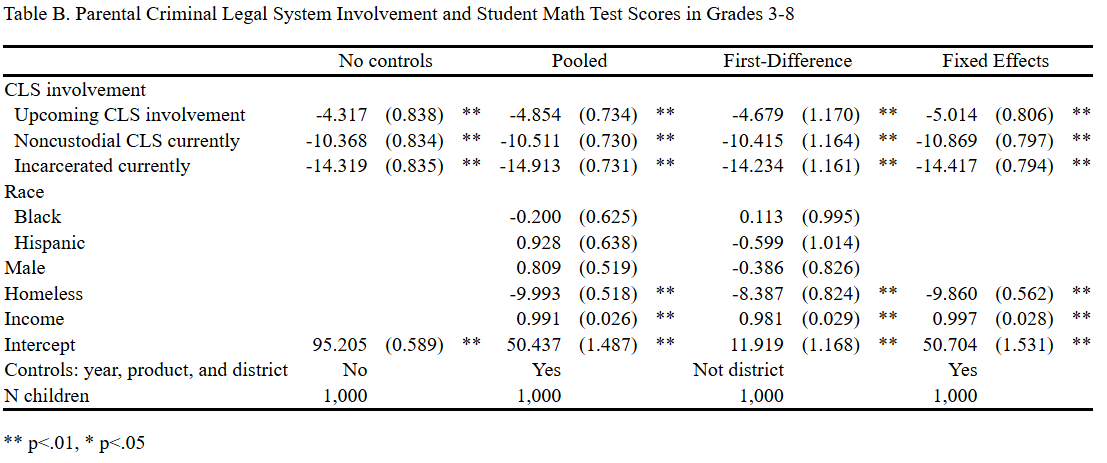
collect title "Table B. Parental Criminal Legal System Involvement and Student Math Test Scores in Grades 3-8"
collect preview
Table B. Parental Criminal Legal System Involvement and Student Math Test Scores in Grades 3-8
----------------------------------------------------------------------------------------------------------------------
                                          No controls          Pooled           First-Difference       Fixed Effects
----------------------------------------------------------------------------------------------------------------------
CLS involvement
  Upcoming CLS involvement             -4.317 (0.838) **  -4.854 (0.734) **       -4.679 (1.170) **  -5.014 (0.806) **
  Noncustodial CLS currently          -10.368 (0.834) ** -10.511 (0.730) **      -10.415 (1.164) ** -10.869 (0.797) **
  Incarcerated currently              -14.319 (0.835) ** -14.913 (0.731) **      -14.234 (1.161) ** -14.417 (0.794) **
Race
  Black                                                   -0.200 (0.625)           0.113 (0.995)
  Hispanic                                                 0.928 (0.638)          -0.599 (1.014)
Male                                                       0.809 (0.519)          -0.386 (0.826)
Homeless                                                  -9.993 (0.518) **       -8.387 (0.824) **  -9.860 (0.562) **
Income                                                     0.991 (0.026) **        0.981 (0.029) **   0.997 (0.028) **
Intercept                              95.205 (0.589) **  50.437 (1.487) **       11.919 (1.168) **  50.704 (1.531) **
Controls: year, product, and district      No                Yes            Not district                Yes
N children                              1,000              1,000                   1,000              1,000
----------------------------------------------------------------------------------------------------------------------
** p<.01, * p<.05