6 Regression Diagnostics

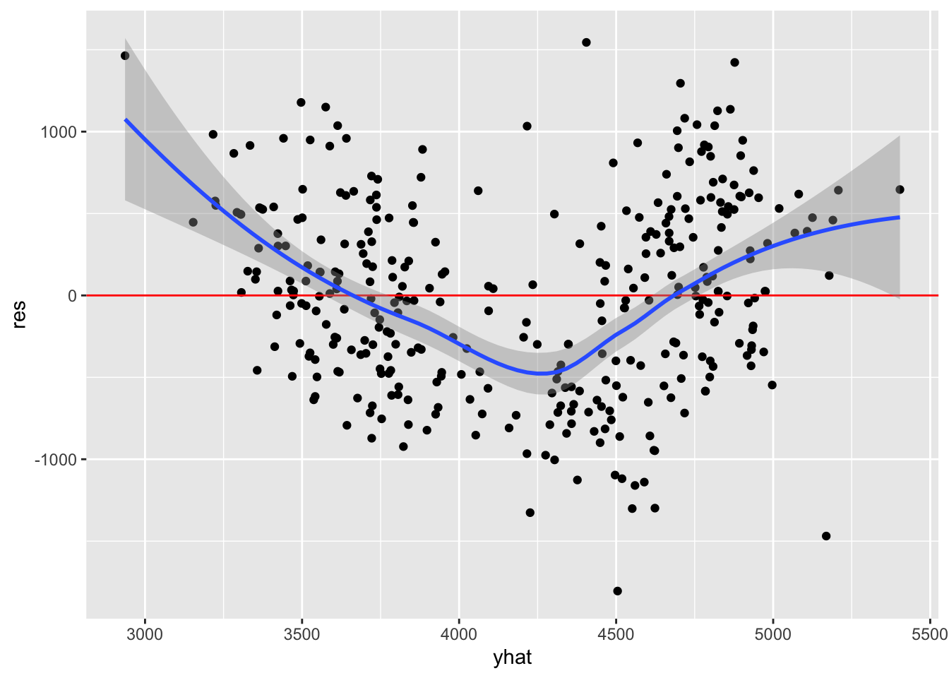
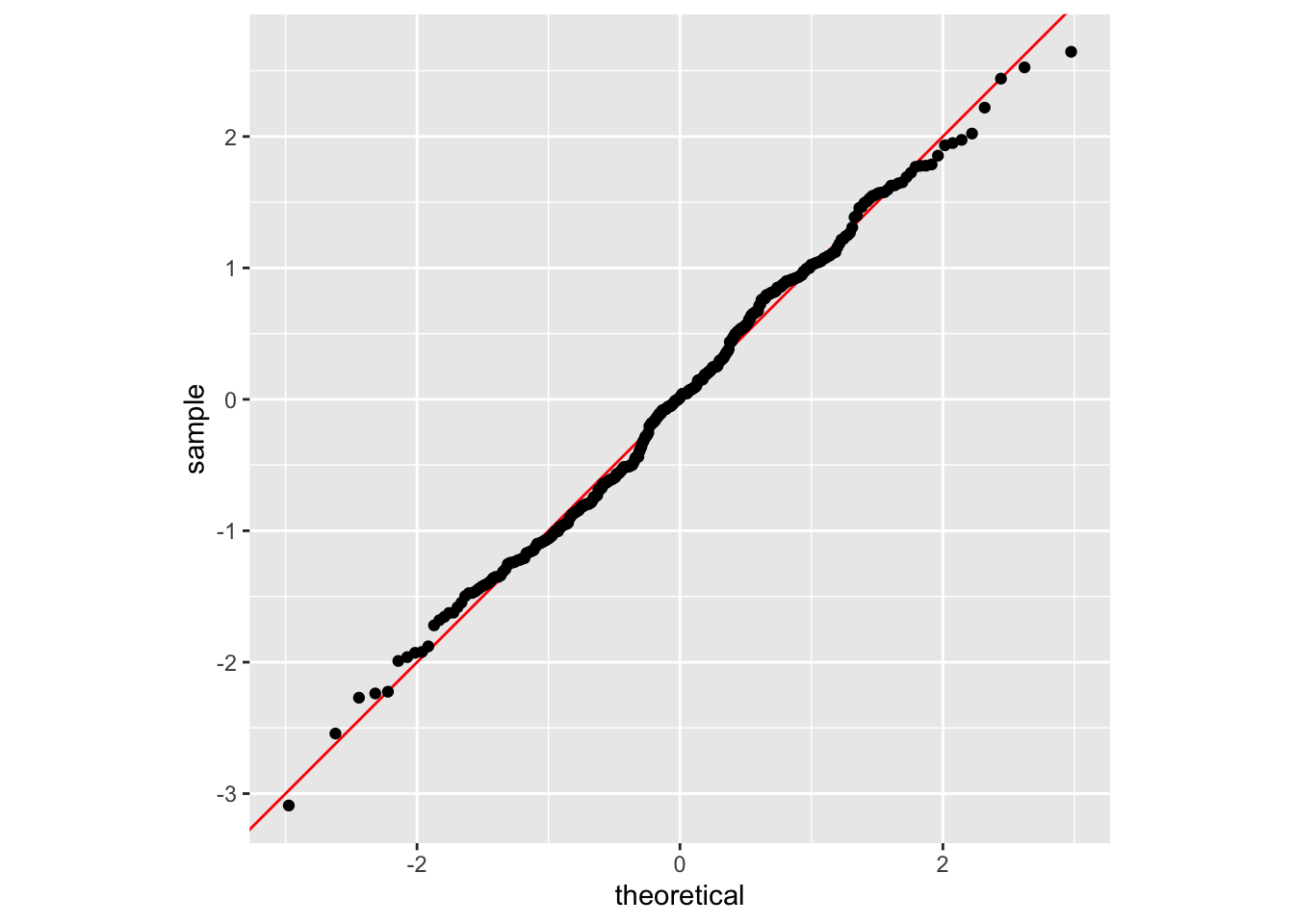
Every statistic you report and model you run relies on assumptions about how the data are distributed. Is it appropriate to report a mean and standard deviation in a table of descriptive statistics? Are the data from the two groups compared in a t-test normally distributed enough? After accounting for control variables in a regression model, are there remaining associations between observations? Are any of the model estimates unduly influenced by a handful of observations?

You do not need to merely assume your model meets certain assumptions. You can actually test assumptions and check for the presence of violations with diagnostic plots.

Diagnostic plots are usually for internal use only. That is, only you or a select few on your research team will ever see them. Because of that, you do not need to spend much time customizing the appearance of these plots. Your only goal is to make plots that are readily interpretable.

This chapter is a mere advertisement for the Regression Diagnostics with R book. This chapter simply shows how to make two plots, while that book systematically explores the assumptions of the linear regression model, discussing in-depth what each one means, why it matters, how to test it, and how to fix violations.

Load the tidyverse and fit a nonsense model predicting penguins’ body mass from their bill length and depth. Because some data is missing, set na.action = na.exclude so that when we extract predicted values and residuals, rows with missing data are returned as NA instead of being omitted. Ideally, you should take a more thoughtful approach to missing data than listwise deletion, but that is another topic and outside the scope of this chapter.

library(tidyverse)

── Attaching core tidyverse packages ──────────────────────── tidyverse 2.0.0 ──
✔ dplyr     1.2.1     ✔ readr     2.2.0
✔ forcats   1.0.1     ✔ stringr   1.6.0
✔ ggplot2   4.0.3     ✔ tibble    3.3.1
✔ lubridate 1.9.5     ✔ tidyr     1.3.2
✔ purrr     1.2.2     
── Conflicts ────────────────────────────────────────── tidyverse_conflicts() ──
✖ dplyr::filter() masks stats::filter()
✖ dplyr::lag()    masks stats::lag()
ℹ Use the conflicted package (<http://conflicted.r-lib.org/>) to force all conflicts to become errors

mod <- lm(body_mass ~ bill_len + bill_dep, penguins, na.action = na.exclude)

Add predicted values and residuals back to the penguins dataframe:

penguins <- 
  penguins |> 
  mutate(yhat = fitted(mod), # predicted values
         res = residuals(mod), # residuals
         res_std = rstandard(mod)) # standardized residuals

Now, partially test the assumption of linearity by plotting the residuals against the fitted values:

ggplot(penguins, 
       aes(x = yhat, 
           y = res)) +
  geom_point() +
  geom_hline(yintercept = 0, color = "red") +
  geom_smooth()

`geom_smooth()` using method = 'loess' and formula = 'y ~ x'

Warning: Removed 2 rows containing non-finite outside the scale range
(`stat_smooth()`).

Warning: Removed 2 rows containing missing values or values outside the scale range
(`geom_point()`).

The systematic departure of the mean line from zero means that the assumption of linearity is violated.

Now, test the assumption of normality by comparing the residual distribution to a normal distribution:

ggplot(penguins, aes(sample = res_std)) +
  geom_abline(color = "red") +
  geom_qq() +
  coord_fixed()

Warning: Removed 2 rows containing non-finite outside the scale range
(`stat_qq()`).

There is no obvious violation of the assumption of normality of residuals.

Learn more in Regression Diagnostics with R.