3 Linearity

What this assumption means: The residuals have mean zero for every value of the fitted values and of the predictors. This means that relevant variables and interactions are included in the model, and the functional form of the relationship between the predictors and the outcome is correct.

Why it matters: Any association between the residuals and fitted values or predictors implies unobserved confounding (i.e., endogeneity), and no causal interpretation can be drawn from the model.

How to diagnose violations: Visually inspect a plot of residuals against fitted values and assess whether the mean of the residuals is zero at every value of \(x\), and use the RESET to test for misspecification.

How to address it: Modify the model, fit a generalized linear model, or otherwise account for endogeneity (e.g., instrumental variables analysis).

3.1 Example Model

If you have not already done so, download the example dataset, read about its variables, and import the dataset into R.

Then, use the code below to fit this page’s example model.

acs <- readRDS("acs2019sample.rds")
mod <- lm(income ~ age + commute_time + education, acs, na.action = na.exclude)

3.2 Statistical Tests

Use the Ramsey Regression Equation Specification Error Test (RESET) to detect specification errors in the model. It was also created in 1968 by a UW-Madison student for his dissertation! The RESET performs a nested model comparison with the current model and the current model plus some polynomial terms, and then returns the result of an F-test. The idea is, if the added non-linear terms explain variance in the outcome, then there is a specification error of some kind, such as the failure to include some curvilinear term or the use of a general linear model where a generalized linear model should have been used.

A significant p-value from the test is not an indication to thoughtlessly add several polynomial terms. Instead, it is an indication that we need to further investigate the relationship between the predictors and the outcome.

To perform the RESET, load the lmtest library. The default of the resettest() function is to test the addition of squared and cubed fitted values.

library(lmtest)
resettest(mod)

## 
##  RESET test
## 
## data:  mod
## RESET = 7.598, df1 = 2, df2 = 2306, p-value = 0.0005141

Considering our original formula of income ~ age + commute_time + education, we could reproduce the default of resettest() as,

anova(mod,
      lm(income ~ age + commute_time + education + I(fitted(mod)^2) + I(fitted(mod)^3), acs))

## Analysis of Variance Table
## 
## Model 1: income ~ age + commute_time + education
## Model 2: income ~ age + commute_time + education + I(fitted(mod)^2) + 
##     I(fitted(mod)^3)
##   Res.Df        RSS Df  Sum of Sq     F    Pr(>F)    
## 1   2308 6.0517e+12                                  
## 2   2306 6.0121e+12  2 3.9619e+10 7.598 0.0005141 ***
## ---
## Signif. codes:  0 '***' 0.001 '**' 0.01 '*' 0.05 '.' 0.1 ' ' 1

The power argument can take other numbers to produce the polynomials (the default is 2:3), and type can be changed from the default fitted to regressors in order to add polynomial terms for each predictor.

# add squared, cubic, and quartic terms for the fitted values
resettest(mod, power = 2:4)

## 
##  RESET test
## 
## data:  mod
## RESET = 5.1591, df1 = 3, df2 = 2305, p-value = 0.001485

# add squared and cubic terms for all of the predictors
resettest(mod, type = "regressor")

## 
##  RESET test
## 
## data:  mod
## RESET = 8.4363, df1 = 4, df2 = 2304, p-value = 9.369e-07

3.3 Visual Tests

Plot the residuals against the fitted values and predictors. Add a conditional mean line. If the mean of the residuals deviates from zero, this is evidence that the assumption of linearity has been violated.

First, add predicted values (yhat) and residuals (res) to the dataset.

library(dplyr)
acs <-
  acs |> 
  mutate(yhat = fitted(mod),
         res = residuals(mod))

Now, plot the residuals and fitted values. Add a horizontal line with geom_hline() as the reference line, and add a conditional mean line with geom_smooth().

library(ggplot2)
ggplot(acs, aes(yhat, res)) +
  geom_point() +
  geom_hline(yintercept = 0, color = "red") +
  geom_smooth()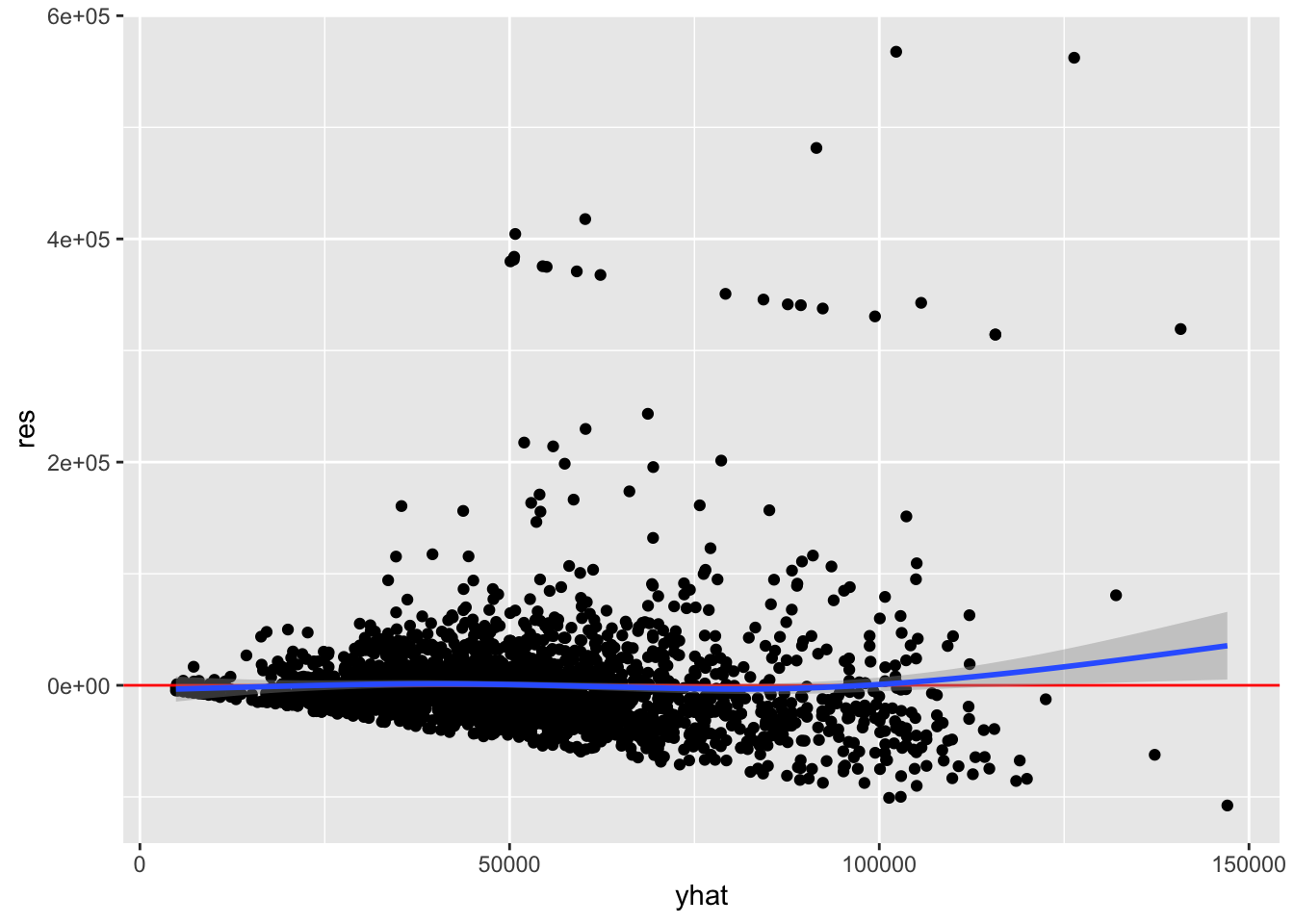

All we are looking for here is whether the conditional mean line deviates from the horizontal reference line, and the two lines overlap for the most part. Although there is an upward trend on the right, very few points exist there so some deviation is expected. Overall, it does not look like there is evidence that the assumption of linearity has been violated.

However, we should be concerned about the fan-shaped residuals that increase in variance from left to right. This is discussed in the chapter on homoscedasticity.

We must also check the residuals against each of the predictors. We will just check age here.

ggplot(acs, aes(age, res)) +
  geom_point() +
  geom_hline(yintercept = 0, color = "red") +
  geom_smooth()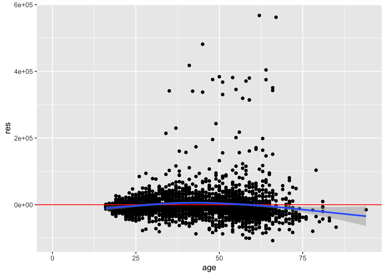

The mean of the residuals is negative on the left, positive in the middle, and again negative on the right. There is evidence for non-linearity with respect to the age variable.

Now, check the residual variance against a categorical predictor, education.

Adding a conditional mean line with a categorical variable requires extra steps in R:

If the categorical variable is a factor, use as.numeric(var) to make it numeric. If it is a character, make it a factor and then numeric with as.numeric(as.factor(var)).
Use stat_summary() with additional arguments, instead of geom_smooth().

ggplot(acs, aes(as.numeric(education), res)) +
  geom_point() +
  geom_hline(yintercept = 0, color = "red") +
  stat_summary(geom = "line", fun = mean, color = "blue", size = 1.5)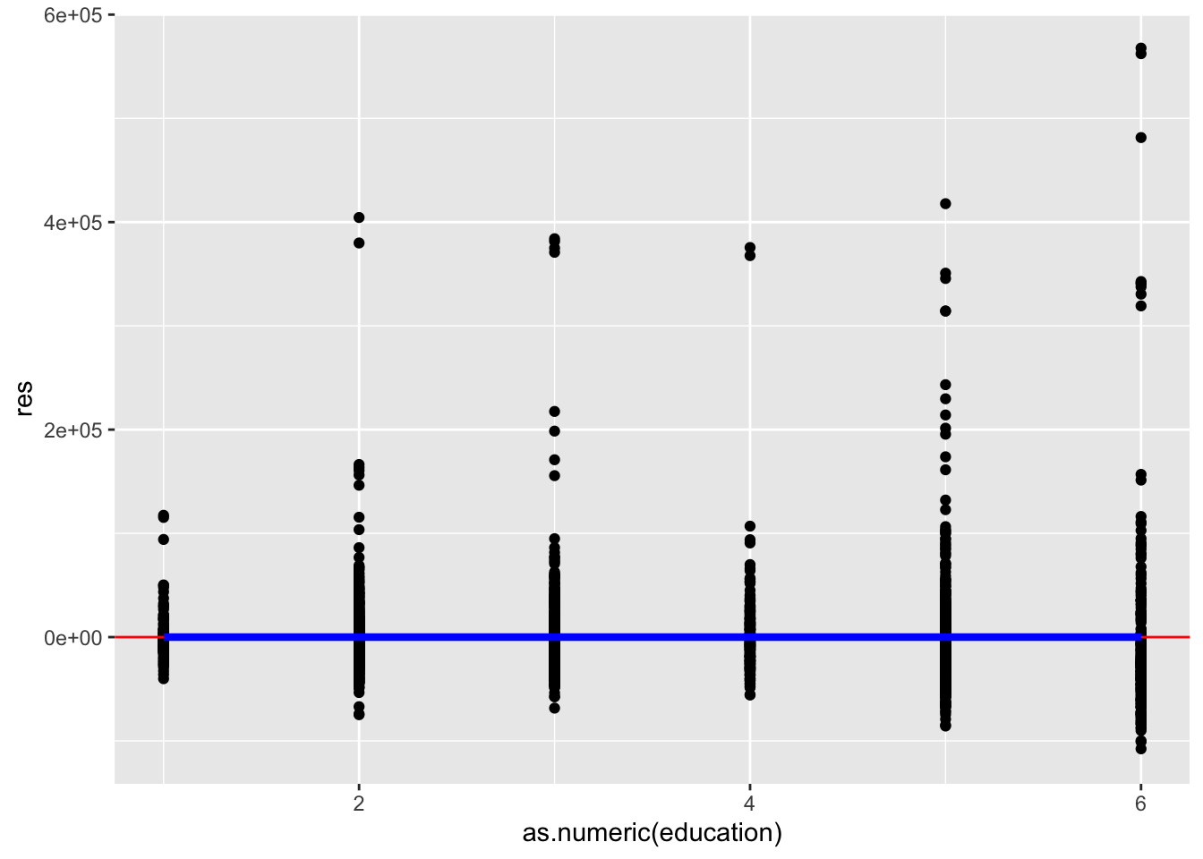

This plot looks good. The mean of the residuals looks to be exactly zero for every level of education.

Optionally, we can also plot the residuals against other variables not included in the model, to see if they correlate with the residuals.

We can try plotting the residuals against hours_worked, which was not in the model.

ggplot(acs, aes(hours_worked, res)) +
  geom_point() +
  geom_hline(yintercept = 0, color = "red") +
  geom_smooth()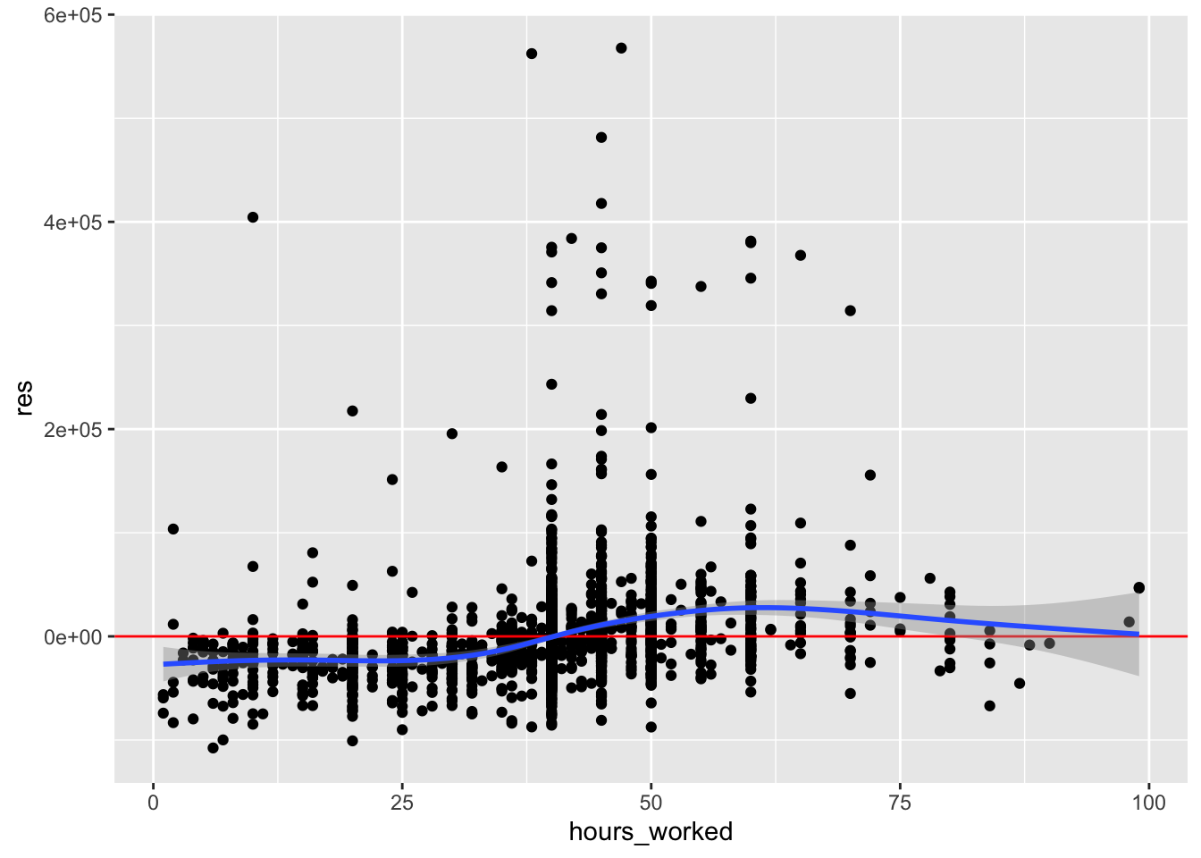

The conditional mean increases from left to right, suggesting a positive relationship. If we have a good theoretical reason to include this variable in our model, we could add it.

3.4 Corrective Actions

We can address non-linearity in one or more ways:

Check the other regression assumptions, since a violation of one can lead to a violation of another.
Modify the model formula by adding or dropping variables or interaction terms.
- Do not simply add every possible variable and interaction in an attempt to explain more variance. Carelessly adding variables can introduce suppressor effects or collider bias.
Add polynomial terms to the model (squared, cubic, etc.).
Fit a generalized linear model.
Fit an instrumental variables model in order to account for the correlation of the predictors and residuals.

After you have applied any corrections or changed your model in any way, you must re-check this assumption and all of the other assumptions.