4 Saving Plots

Load the libraries necessary for this page:

library(tidyverse)

This chapter will teach you how to save R plots, turning them from an image within RStudio into a file on your computer. Plots created with ggplot will receive primary attention, but options for saving plots created with other packages will also be covered.

Generally speaking, in R, whatever we create and calculate during our session is not available once we end our session. That includes new variables we added to our dataset, models we fit, and plots we created (learn more about saving data objects). To share a plot with somebody else (whether in a homework assignment or journal submission), we first need to save the plot by exporting it as a file.

Three options for saving plots are outlined below:

ggplot’s ggsave() function
Base R’s graphic device functions
RStudio interface

ggsave() has additional options to customize the saved plot, and these are discussed below. The two other methods for saving plots are covered only briefly.

4.1 ggsave (ggplot2 Plots)

If you are creating plots with ggplot, the best option is to use ggsave(), which saves the most recently created ggplot plot. The plot does not need to have been created explicitly with the ggplot() function. Many packages, such as ggeffects() in the chapter on Visualizing Regression Results, use ggplot behind the scenes to draw plots, so ggsave() can be used to save these plots too. However, ggsave() will ignore any plots made with functions from other packages when detecting the last plot, such as plot() or hist() from base.

4.1.1 File Dimensions

The default size of the saved image is equal to the size of Plots pane (the “graphics device”) in RStudio, which not reproducible and likely too small. Instead, manually specify the dimensions when saving the image.

It usually takes a little back-and-forth between selecting dimensions, saving the file, checking the appearance of the saved file, and adjusting the dimensions and geom sizes.

By default, units are specified in inches, but this can be changed.

ggsave("plot.pdf", width = 6,      height = 4)
ggsave("plot.pdf", width = 15.24,  height = 10.16, units = "cm")
ggsave("plot.pdf", width = 152.4,  height = 101.6, units = "mm")

Plot elements like text and geom are constant sizes. No matter how big or small the plot, by default, axis labels are always size 11 font and geom_point() points are always 1.5 mm. The consequence of this is that the relative size of these elements depends on the plot size. If the plot is too small, the text is too big, but if the plot is too big, the text is too small to be readable.

Observe the results of saving the following plot with dimensions that are either too small or too big:

ggplot(mtcars, 
       aes(x = wt, 
           y = mpg)) +
  geom_point()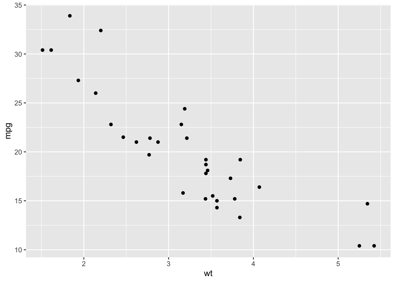

ggsave("too-small.png", width = 1.5, height = 1)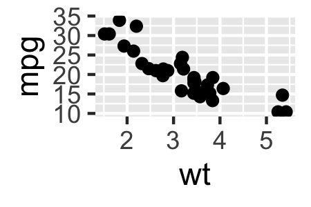

ggsave("too-large.png", width = 12, height = 8)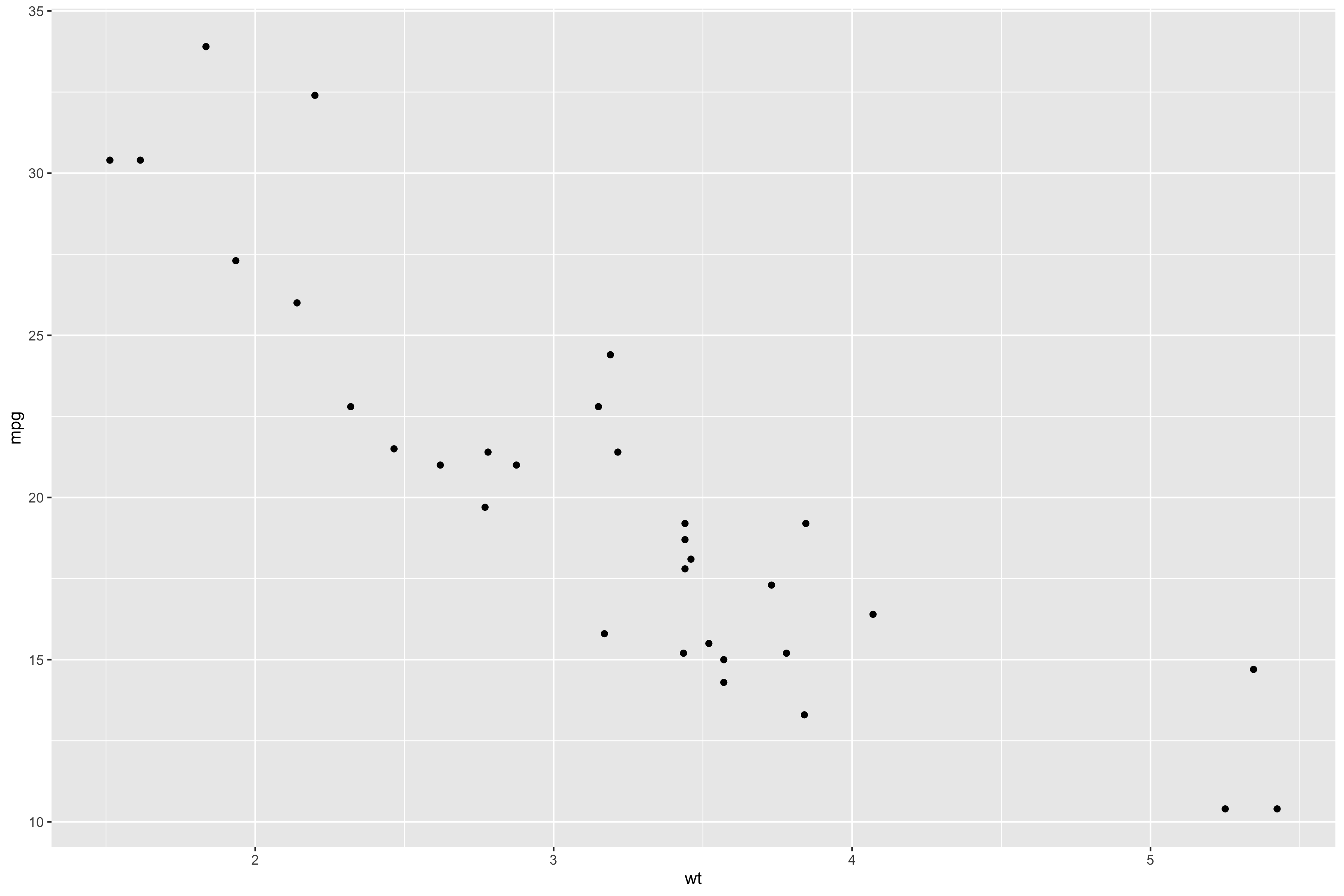

What size should you use as a default?

width = 6, height = 4 is usually fine for inserting into a Microsoft Word document or emailing to colleagues, but once you add more elements or need to be displayed in a different size, you need to pick new dimensions.

If you have a simple plot that needs to fit in one column in a journal submission, you may need smaller than 6x4.

If you have a more complex plot with a legend or facets, or if you need to present the plot at a larger size, such as a whole page or on a poster at a conference, you will need to make it larger than 6x4.

4.1.2 File Extensions

ggsave() supports several file extensions, which can be found in ?ggsave next to the device argument and are also listed in the following table, along with whether that extension is vectorized and supports semi-transparency (“alpha”):

Extension	Vectorized	Alpha support
.bmp	No	Yes
.eps	Yes	No
.jpeg	No	Yes
.pdf	Yes	Yes
.png	No	Yes
.ps	Yes	No
.svg	Yes	Yes
.tex	Yes	Yes
.tiff	No	Yes
.wmf	Partial	No

The file extension can be specified simply as part of the file name, as in ggsave("plot.png").

For most purposes, you should save the file with a PDF, PNG, or TIFF extension, depending on how you would like to use it. When including a plot as a figure in a journal submission, review the journal’s requirements. If you need to insert it into a document like Microsoft Word or a poster, you should use PNG or TIFF.

PDF files excel in quality and compatibility with other applications, making it the preferred file type. However, some situations require other file extensions to be used. If that is the case, it is important to know about image vectorization and alpha.

4.1.2.1 Vector Graphics

Images that are vectorized contain instructions for how an image is to be drawn: draw a black line from point A to point B, write the number “10” at point C, and so on.

Images that are not vectorized are coded as tables of color values: the pixel in picture[1, 1] is white, picture[1, 2] is black, picture[1, 3] is dark blue, and so on. Non-vectorized images are also called rasterized or bitmap images.

Because of this difference, vectorized images can be rescaled without any effect on image quality. On the other hand, if we make a non-vectorized image too large, we might be able to see individual pixels (i.e., pixelization).

To see this, we can save the following plot in a vectorized format (PDF) and a non-vectorized format (PNG).

ggplot(mtcars, 
       aes(x = wt, 
           y = mpg)) + 
  geom_point() +
  geom_abline(intercept = 10, slope = 3, color = "red") +
  geom_smooth(se = F)

`geom_smooth()` using method = 'loess' and formula = 'y ~ x'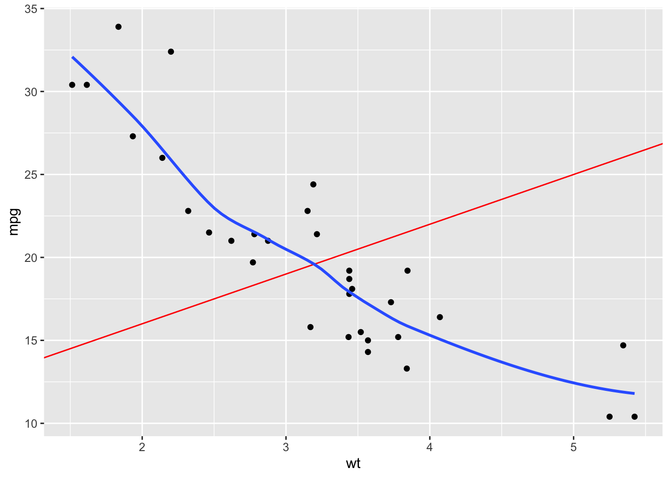

ggsave("plot.pdf")
ggsave("plot.png")

Compare the image quality if we zoom into the “10” on the y-axis of the two plots:

PDF:

PNG:

At this level, we can see the individual pixels of the PNG image, while the PDF image retains its quality.

Understanding how images are encoded is important when presenting large plots, such as on posters or in presentations. Using a vectorized image format is a good way to ensure your plots retain their quality when enlarged. If that is not possible, save the image with sufficient size and resolution.

4.1.2.2 Resolution

When saving PNGs, TIFFs, or other non-vectorized image types, the resolution can be specified with dpi, dots (printed pixels) per inch. A higher dpi results in a larger file since more data is encoded in it, but it produces a clearer image. The default dpi is 300, but some journals may require a higher number, such as 600.

ggsave("plot.tiff", dpi = 600)

4.1.2.3 Alpha Support

The alpha parameter controls the degree of transparency. PDF, PNG, and TIFF all have alpha support.

Many geoms can be set to be partially transparent with the alpha argument, and geom_smooth() contains a semi-transparent confidence band by default. alpha can range from 0 to 1, where 0 is completely transparent (and therefore invisible) and 1 is opaque.

In the code below, alpha = .5 makes all of the points semi-transparent.

ggplot(mtcars, aes(x = wt, y = mpg)) +
  geom_point(alpha = .5) +
  geom_smooth()

`geom_smooth()` using method = 'loess' and formula = 'y ~ x'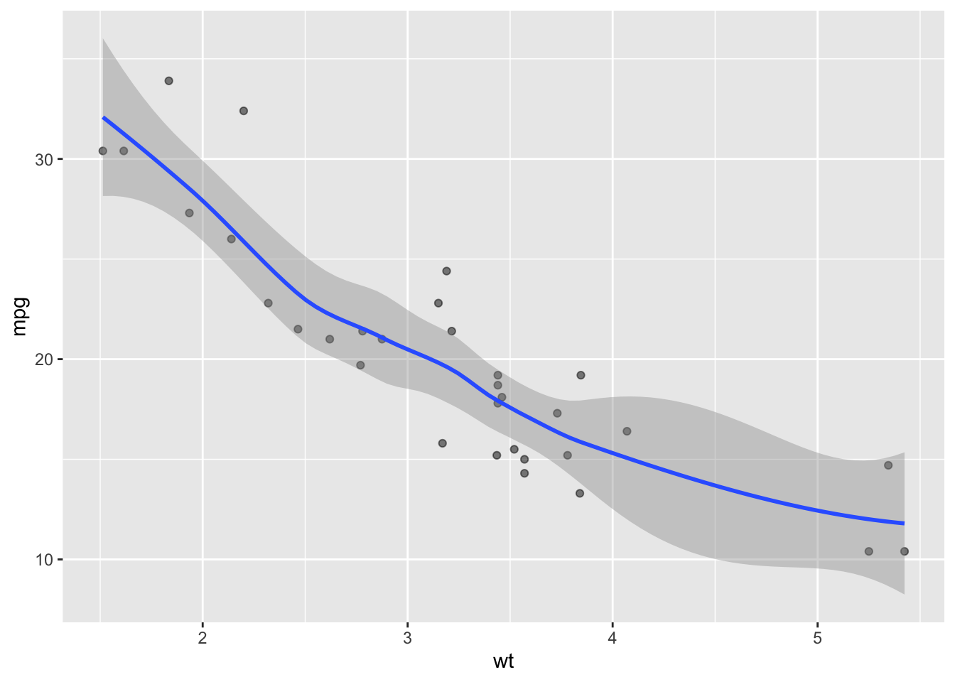

File extensions without alpha support, such as EPS, will simply omit features that are not fully opaque.

ggsave("plot.eps")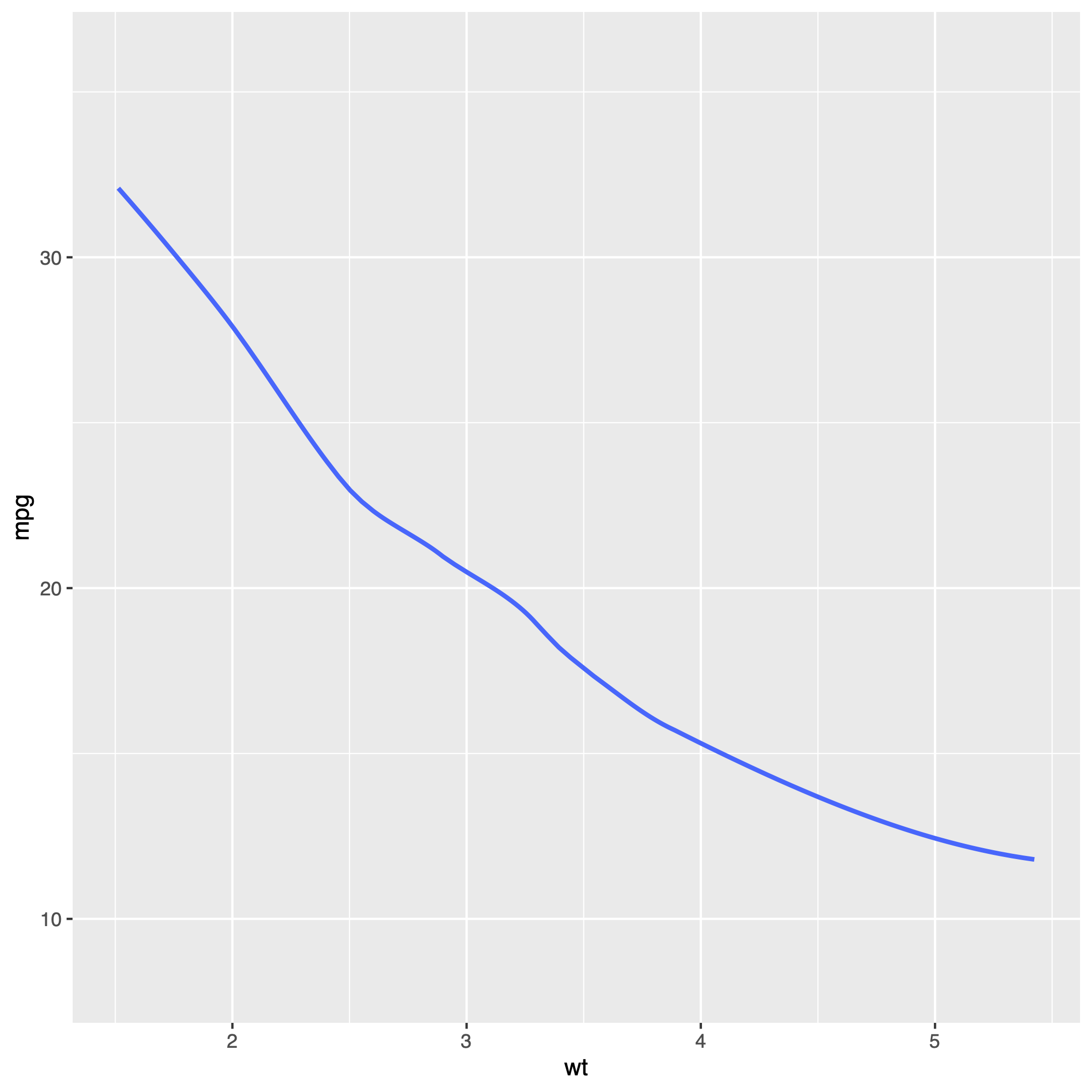

All of the semi-transparent points and the confidence band are missing!

4.2 Other Options for Saving Plots

4.2.1 Graphics Devices (Base R Plots)

If we create plots outside of ggplot (with plot(), hist(), boxplot(), etc.), we cannot use ggsave() to save our plots since it only supports plots made with ggplot.

Base R provides a way to save these plots with its graphic device functions. Instead of a two step process of (1) creating a plot and then (2) saving it as with ggsave(), we have three steps when using base R:

Specify the file extension and properties (size, resolution, etc.).
- Supported extensions: bmp(), jpeg(), png(), tiff(), and pdf()
- Units can be specified in pixels (px, the default for the first four extensions), inches (in, the default for pdf()), centimeters (cm), or millimeters (mm).
Create the plot with base R, ggplot, or any other plotting package.
- Note: Step 1 instructs R to plot in a different graphics device, so the plot will not be shown in the Plots pane
Signal that the plot is finished and save it by running dev.off().

Here are two examples, one made with ggplot() and saved as a PNG, and one made with base R’s plot() and saved as a PDF.

png(filename = "plot3.png", width = 6, height = 4, units = "in", res = 300)
ggplot(mtcars, 
       aes(x = wt, 
           y = mpg)) + 
  geom_point() +
  geom_abline(intercept = 10, slope = 3, color = "red")
dev.off()

pdf(file = "plot4.pdf", width = 6, height = 4)
plot(mtcars$wt, mtcars$mpg)
abline(a = 10, b = 3, col = "red")
dev.off()

4.2.2 RStudio Interface

RStudio provides a point-and-click method to save plots in the Plots pane. This method is not recommended, however, because it leaves no record and is thus not reproducible, but it is at times convenient to quickly save and share an image.

To save a plot in this way, first create the plot, and then click on Export in the Plots pane.

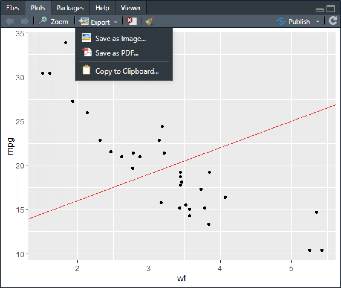
Selecting Save as Image… yields the dialog below. Several image formats are supported: PNG, JPEG, TIFF, BMP, SVG, and EPS. The plot dimensions (in pixels), path, and name can be chosen here.

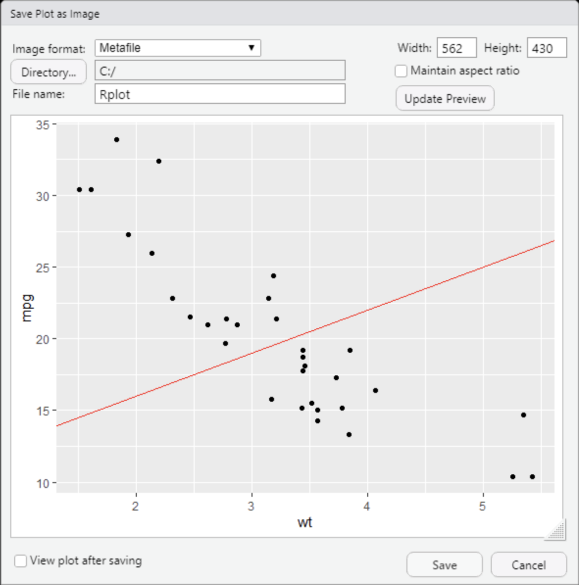
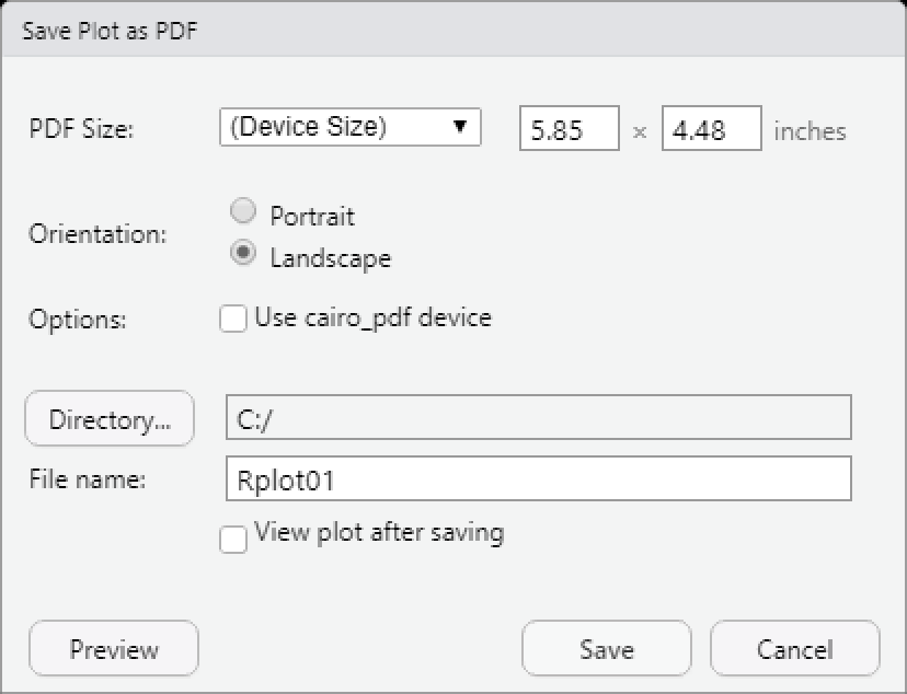
In the Export menu, selecting Save as PDF… brings up the menu below, where the plot dimensions (in inches), path, and name can be specified.