library(tidyverse)
library(ggeffects)
library(ggpubr)
library(ggrepel)7 Visualizing Regression Results
This chapter will teach you how to use ggpredict() and plot() to visualize the marginal effects of one or more variables of interest in linear and logistic regression models. You will learn how to specify predictor values and how to fix covariates at specific values, in addition to options for customizing plots.
Marginal means are predicted outcomes given certain constraints, and a marginal effect is the predicted change in the outcome after varying a variable of interest while holding others constant.
As our models grow in complexity and dimensionality, we face increasing difficulty in interpreting coefficients. Visualizing margins helps us better understand and communicate our model results.
To begin, load these packages. ggeffects has the ggpredict() function, which we will use to calculate margins.
Load a sample of the 2019 American Community Survey. The variables in this dataset are described in Regression Diagnostics with R.
acs <- readRDS(url("https://sscc.wisc.edu/sscc/pubs/data/RegDiag/acs2019sample.rds"))Fit a linear model predicting income from age, education, and their interaction; hours_worked per week; and sex.
mod <- lm(income ~ age * education + hours_worked + sex, acs)Now, suppose we want to understand the marginal effect of age for females with a bachelor’s degree who work 40 hours per week.
View the model estimates with summary():
summary(mod)
Call:
lm(formula = income ~ age * education + hours_worked + sex, data = acs)

Residuals:
    Min      1Q  Median      3Q     Max
-104651  -20303   -5457   10053  575865

Coefficients:
                                 Estimate Std. Error t value Pr(>|t|)
(Intercept)                     -14651.75    7303.23  -2.006 0.044933 *
age                                321.88     188.29   1.709 0.087479 .
educationHigh school             -2538.18    8806.58  -0.288 0.773204
educationSome college           -11156.06    9145.48  -1.220 0.222629
educationAssociate's degree       6956.78   12208.20   0.570 0.568829
educationBachelor's degree       -2617.29   10355.82  -0.253 0.800491
educationAdvanced degree         43542.41   15015.65   2.900 0.003764 **
hours_worked                      1061.12      72.49  14.637  < 2e-16 ***
sexFemale                       -15115.84    1966.42  -7.687 2.08e-14 ***
age:educationHigh school           174.06     213.52   0.815 0.415029
age:educationSome college          505.64     223.04   2.267 0.023466 *
age:educationAssociate's degree    154.85     280.84   0.551 0.581415
age:educationBachelor's degree     813.06     246.26   3.302 0.000973 ***
age:educationAdvanced degree       329.19     316.10   1.041 0.297781
---
Signif. codes:  0 '***' 0.001 '**' 0.01 '*' 0.05 '.' 0.1 ' ' 1

Residual standard error: 49320 on 2747 degrees of freedom
  (2239 observations deleted due to missingness)
Multiple R-squared:  0.2391,    Adjusted R-squared:  0.2355
F-statistic: 66.39 on 13 and 2747 DF,  p-value: < 2.2e-16
Our model estimates give us the coefficient estimates and significance tests we have been trained to interpret and report, but they are less useful when we want to calculate expected outcomes.
ggpredict() with plot() provides a visual aid for select terms. The two are complementary; neither can fully replace the other.
ggpredict(mod,
          terms = "age",
          condition = c(education = "Bachelor's degree",
                        hours_worked = 40,
                        sex = "Female")) |>
  plot()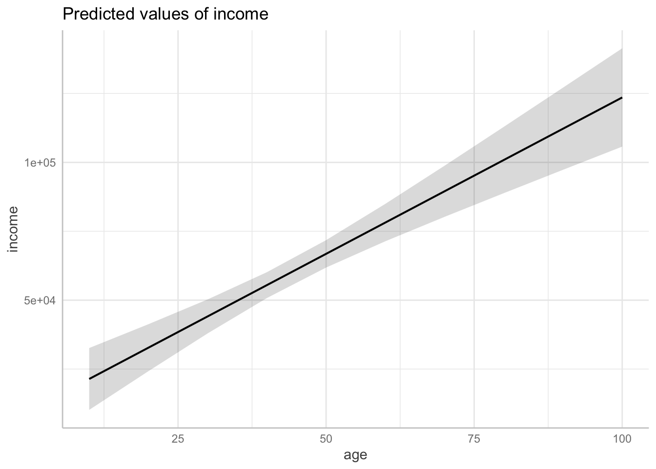
This plot helps us visualize the marginal effect of age on income when we hold education, hours_worked, and sex constant at specific values. The expected increase in income with age appears to be quite substantial.
7.1 Plotting margins
We will continue to plot margins from mod, our regression model fit to the acs dataset.
We will use two functions to create margins plots: ggpredict() and plot(). ggeffects has an additional method for plot() to create margins plots with ggplot. That is to say, these are plots made with ggplot, so we can apply all the techniques for saving and customizing plots covered in other parts of this book.
Two arguments of ggpredict() that we will use to begin are model and terms. model is just the name of our fitted model, mod.
terms takes a character vector of up to five predictor names, but here we will only use three. The three terms are mapped to the ggplot aesthetics of x, group, and facet, in that order.
xis mapped to the x-axisgroups have different lines, colors, and/or shapesfacets are separate sub-plots
The three terms take different types of variables.
xcan be continuous or categoricalgroupandfacetmust be categorical, or they will be made categorical- See Margins at Specific Values to specify how continuous variables are handled (e.g., by using specific values, mean ± SD, etc.)
7.1.1 Terms
Our model has two continuous (age, hours_worked) and two categorical variables (education, sex). We can create a range of plots with different numbers and orders of these variables.
One continuous:
ggpredict(mod,
          terms = c("age")) |>
  plot()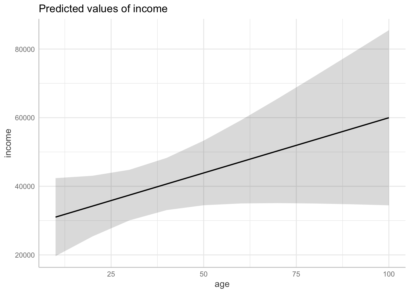
One categorical:
ggpredict(mod,
          terms = c("education")) |>
  plot()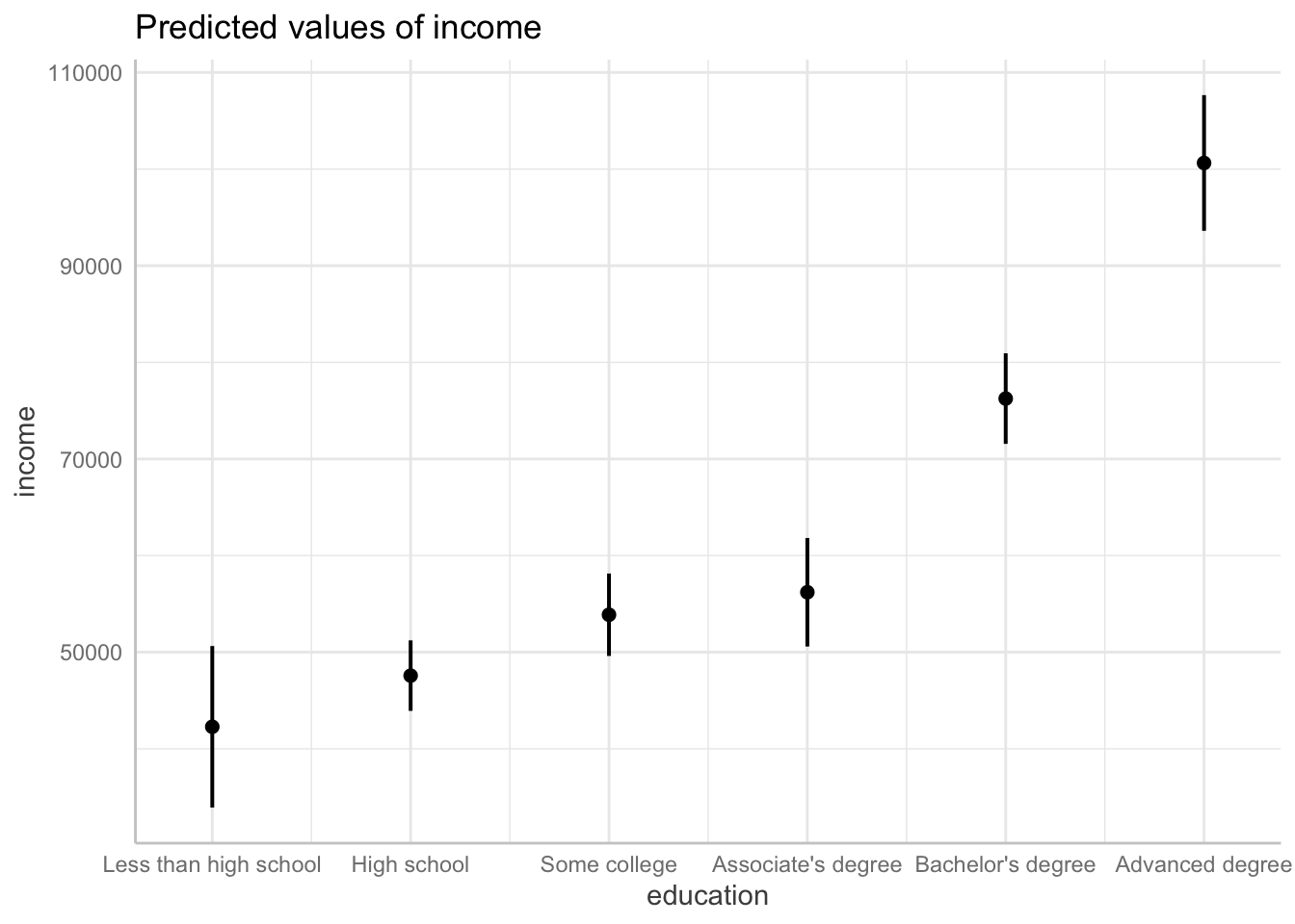
Two continuous:
ggpredict(mod,
          terms = c("age", "hours_worked")) |>
  plot()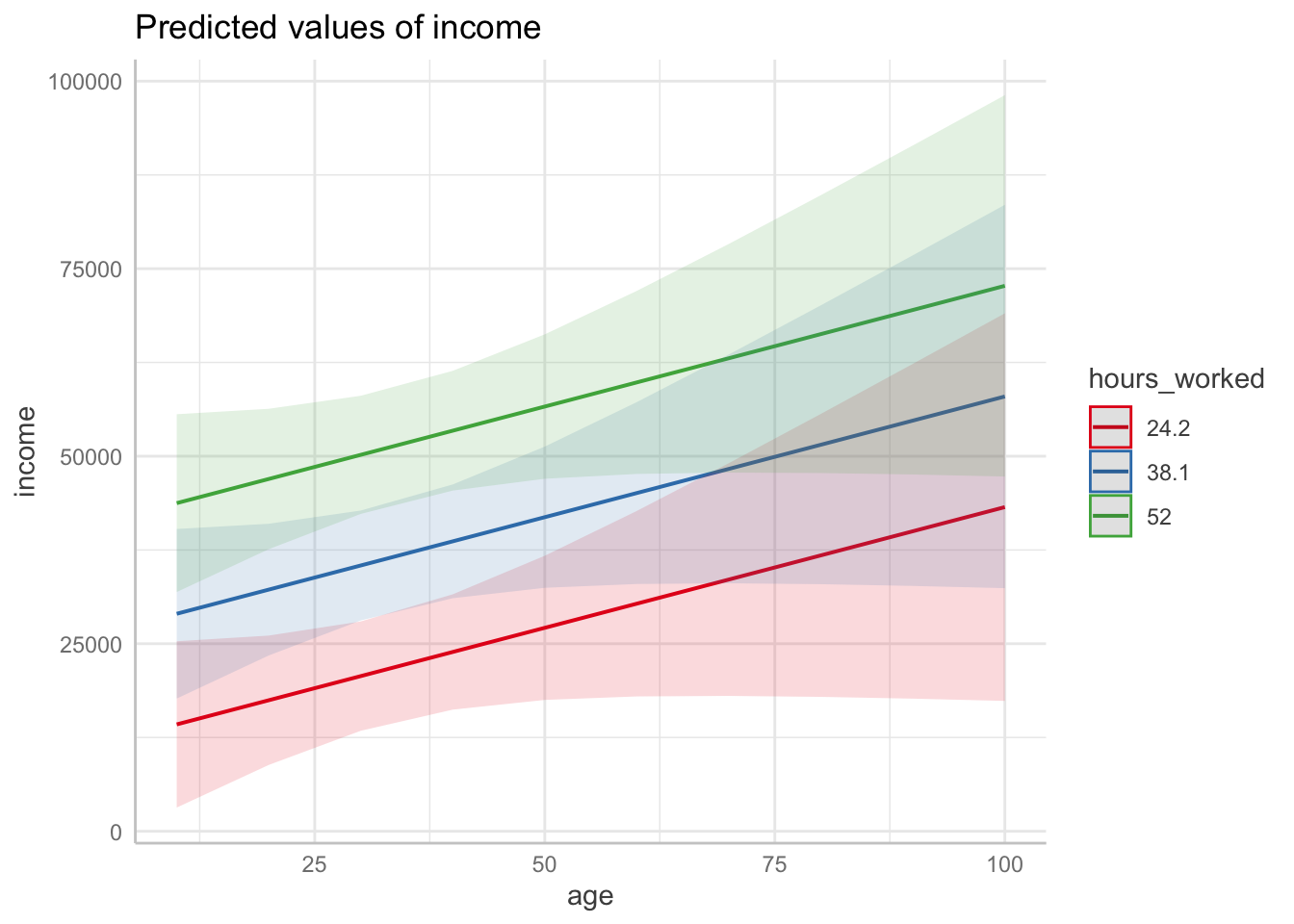
Two categorical:
ggpredict(mod,
          terms = c("education", "sex")) |>
  plot()
Ignoring unknown labels:
• linetype : "sex"
• shape : "sex"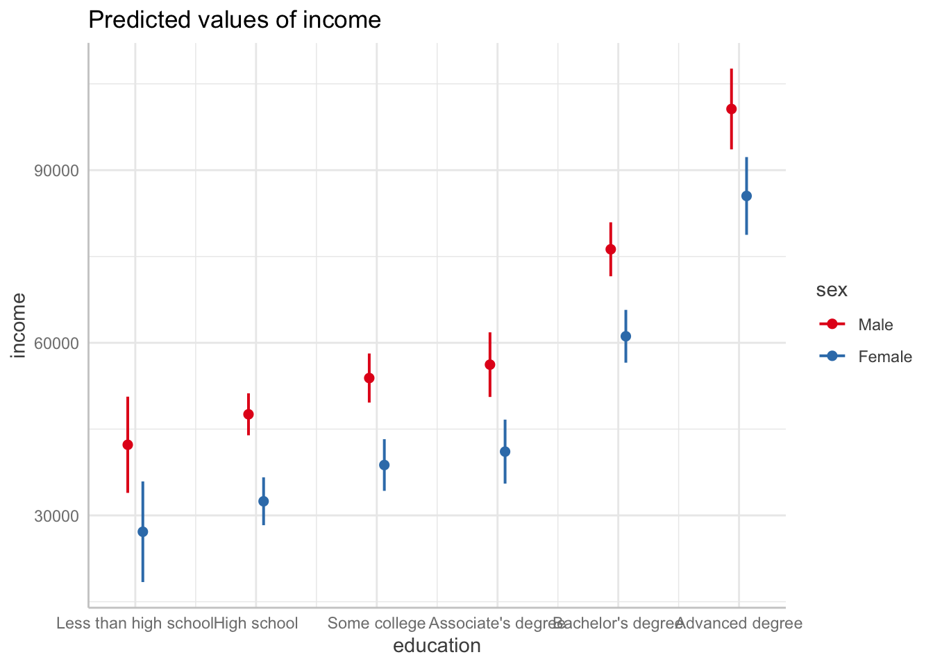
One continuous then one categorical:
ggpredict(mod,
          terms = c("age", "sex")) |>
  plot()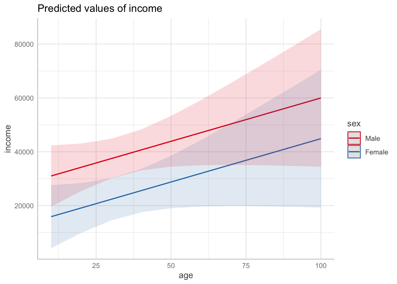
One categorical then one continuous. Compare this plot to the previous plot, noticing how age is turned into a categorical variable since it is the group term.
ggpredict(mod,
          terms = c("sex", "age")) |>
  plot()
Ignoring unknown labels:
• linetype : "age"
• shape : "age"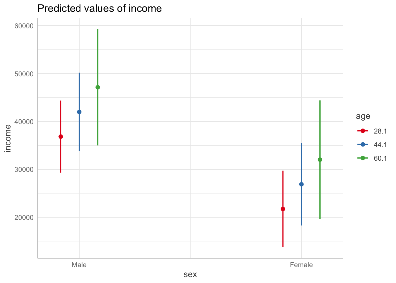
One continuous then two categorical:
ggpredict(mod,
          terms = c("age", "sex", "education")) |>
  plot()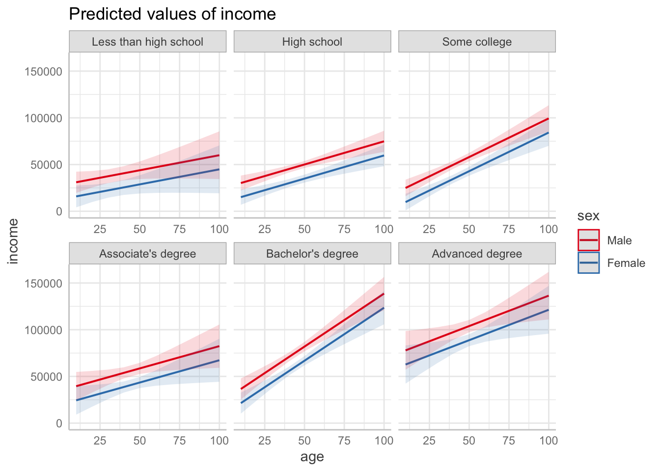
7.2 Margins at specific values
7.2.1 Of predictors
ggpredict() will by default plot margins for all values of our x term and certain values of our group and facet terms. We may want to reduce the range of continuous variables or examine margins for only some of the values a categorical variable can take.
To plot margins at specific values of terms, specify the terms as var [values], where var is the variable name and values can take on one of several forms:
- Comma-separated values:
[20, 40, 60, 80]- For factors, specify the levels of interest without quotes:
[High school, Bachelor's degree]
- For factors, specify the levels of interest without quotes:
- Sequence with
::[30:40]- Optionally, add a step size:
[20:80, by=20]
- Optionally, add a step size:
- Mean ± one standard deviation (default for continuous variables when they are
grouporfacet):[meansd] - First quartile, median, and third quartile:
[quart2]
See more options at ?values_at.
We can plot margins for values of 20 to 80 for age and high school and bachelor’s degree for education:
ggpredict(mod,
          terms = c("age [20:80]",
                    "education [High school, Bachelor's degree]")) |>
  plot()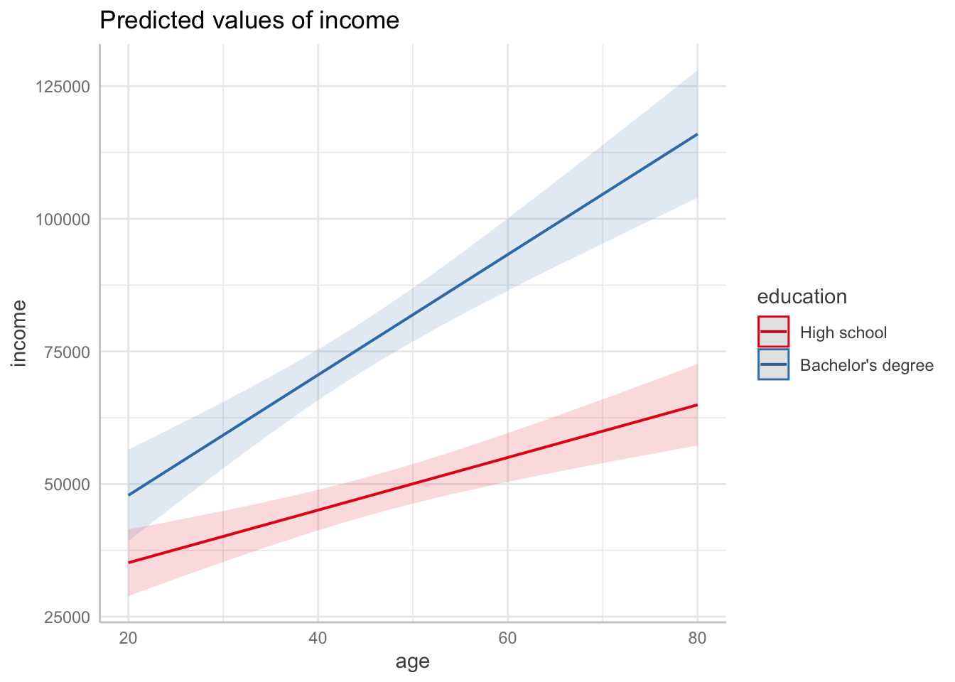
7.2.2 Of covariates
Recall that margin effects are predicted changes in the outcome while holding all else constant. We should ask, held constant at what value? ggpredict() by default will set numeric terms to their means and factor terms to their reference level.
To change these, use the condition argument of ggpredict(). Supply it with a vector of var = value pairs.
The plot below shows the marginal effect of age when education is high school and hours_worked is 45.
ggpredict(mod,
          terms = c("age"),
          condition = c(education = "High school",
                        hours_worked = 45)) |>
  plot()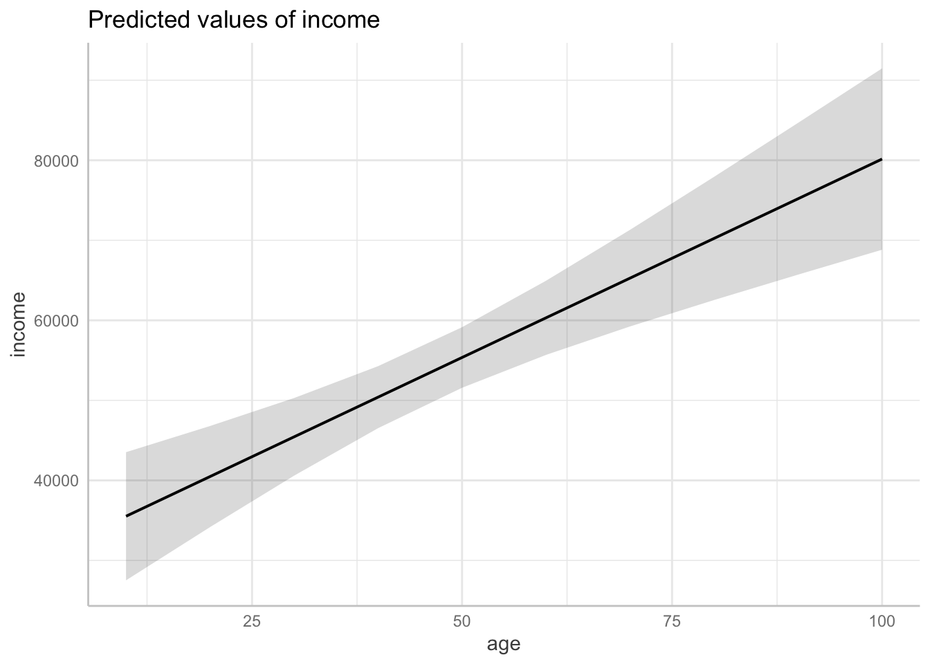
The other term in our model is sex, a factor. We did not specify a condition, so it was fixed at its reference level (male).
We can confirm this by adding a condition to fix sex to its reference level, and we can see the plot is exactly the same:
ggpredict(mod,
          terms = c("age"),
          condition = c(education = "High school",
                        hours_worked = 45,
                        sex = "Male")) |>
  plot()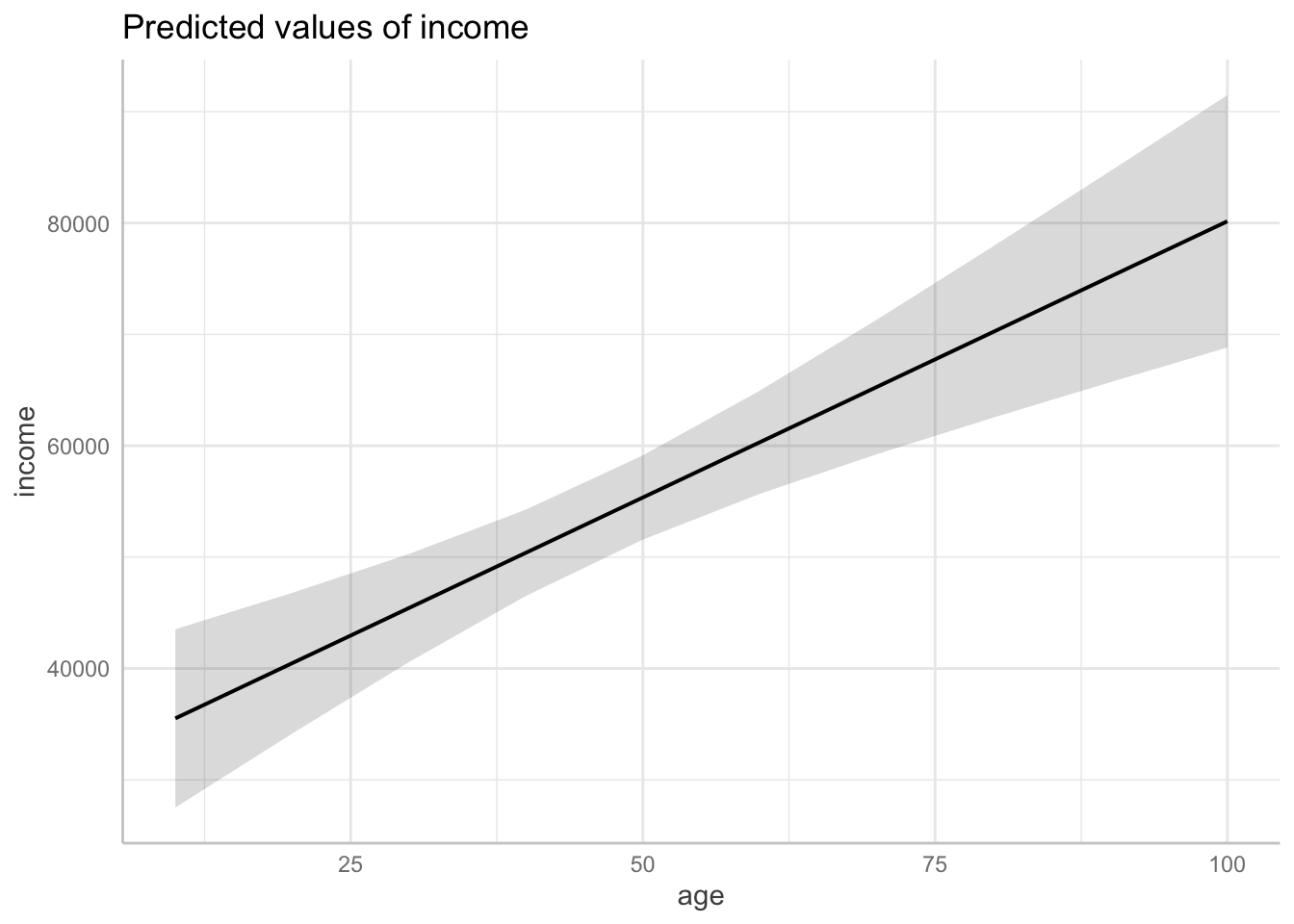
7.3 Customizing plot appearance
The plot() method from ggeffects includes some options for customization. For further fine-tuning, we can modify our margins plots with ggplot functions like labs() and theme() since plot() uses ggplot.
7.3.1 Show the data
When we plotted raw data, we chose to show the distribution of the data in addition to a summary statistic (mean or median). When plotting model estimates, it is no different. The regression line or predicted values are summary statistics themselves, typically reflecting the mean. Confidence bands and error bars do hint at the variance, but they are often not enough to communicate the data distribution.
The plot() function has an argument, show_data, that is set to FALSE by default. Setting it to TRUE will plot the raw data:
ggpredict(mod,
          terms = c("age", "sex")) |>
  plot(show_data = T)
Data points may overlap. Use the `jitter` argument to add some amount of
random variation to the location of data points and avoid overplotting.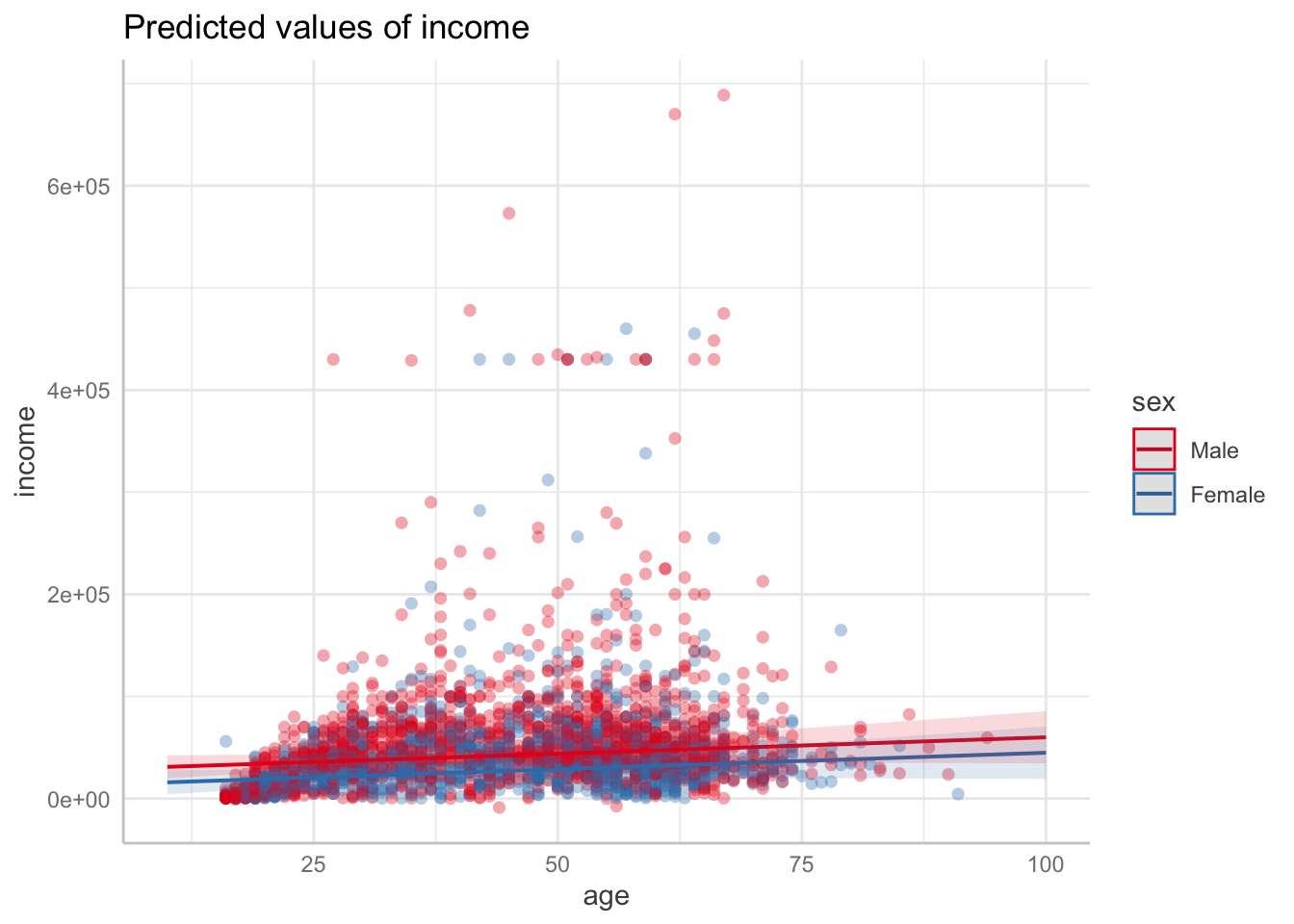
Suddenly the model does not look so good anymore. Part of the problem, if we can call it that, is that the \(R^2\) is only 0.239, and part of the problem (and this part really is a problem) is the residual distribution that is decidedly nonnormal and heteroscedastic. (Check your model assumptions!)
7.3.2 Confidence intervals
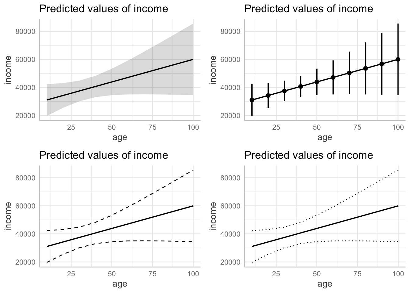
For continuous variables, modify the ci_style argument to get confidence intervals of four types: ribbon (default), errorbar, dash, or dot.
ggarrange(
  ggpredict(mod, terms = c("age")) |> plot(ci_style = "ribbon"),
  ggpredict(mod, terms = c("age")) |> plot(ci_style = "errorbar"),
  ggpredict(mod, terms = c("age")) |> plot(ci_style = "dash"),
  ggpredict(mod, terms = c("age")) |> plot(ci_style = "dot"),
  ncol = 2, nrow = 2
)
Alternatively, confidence intervals can be removed by setting show_ci = F. This works for both continuous and categorical variables.
ggpredict(mod,
          terms = c("age")) |>
  plot(show_ci = F)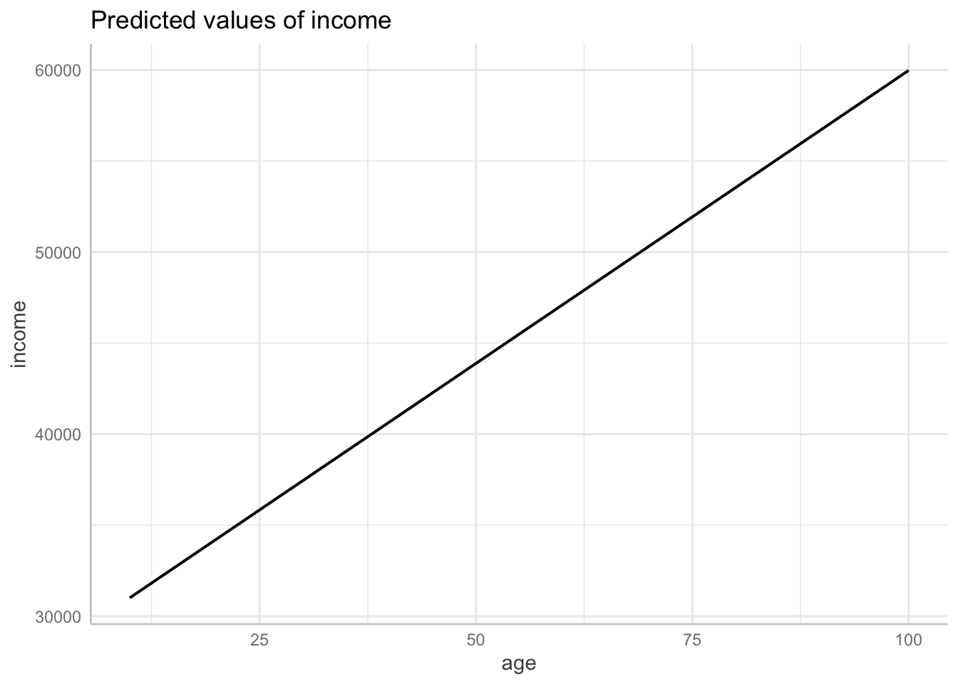
7.3.3 Colors
The group aesthetic is assigned colors, which we can change with the colors argument of plot(). Options include
bwfor black and whitegsfor gray scale- Other presets, which you can find along the y-axis of the plot produced by
show_pals()- Be sure to verify the palette has at least as many colors as the
grouphas levels.
- Be sure to verify the palette has at least as many colors as the
- A vector of color names or codes:
colors = c("red", "green", "#0000ff)- Get color codes from this web app
The default is set1 from show_pals().
For a journal submission, you will most likely need to change your plot to black and white. If your first value in terms is continuous, then your plot will have lines, so a black-and-white group will be mapped onto linetype:
ggpredict(mod,
          terms = c("age", "sex")) |>
  plot(colors = "bw")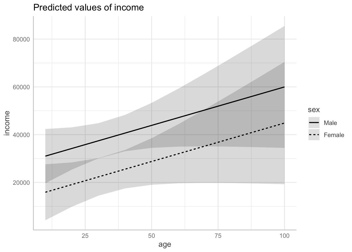
If the first value in terms is categorical, the plot will have points, so a black-and-white group will be mapped onto shape:
ggpredict(mod,
          terms = c("education", "sex")) |>
  plot(colors = "bw")
Ignoring unknown labels:
• linetype : "sex"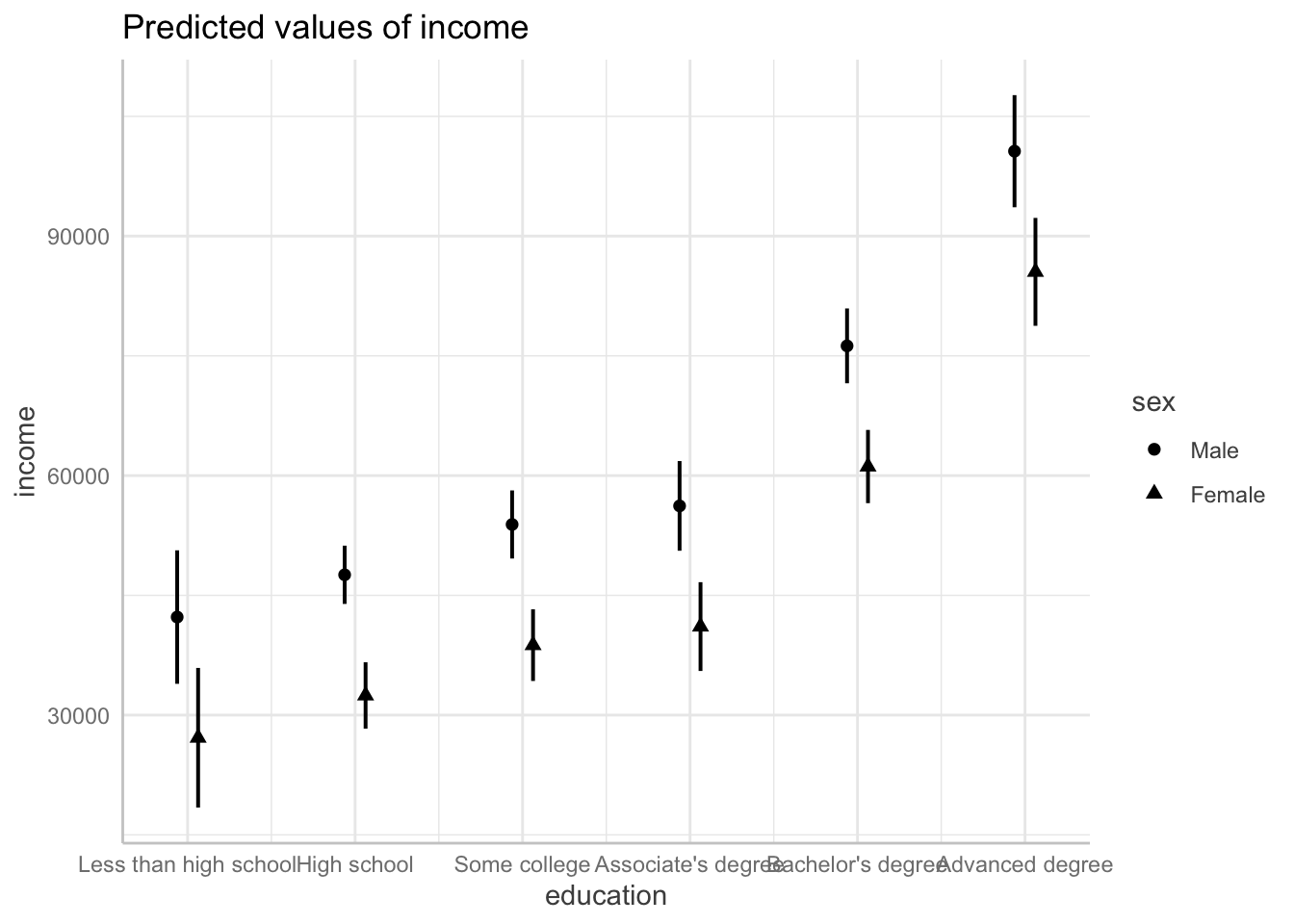
7.3.4 Themes
plot() uses its own custom ggplot theme.
Add use_theme = F to return to ggplot’s default theme.
ggpredict(mod, terms = c("age")) |> plot(use_theme = F)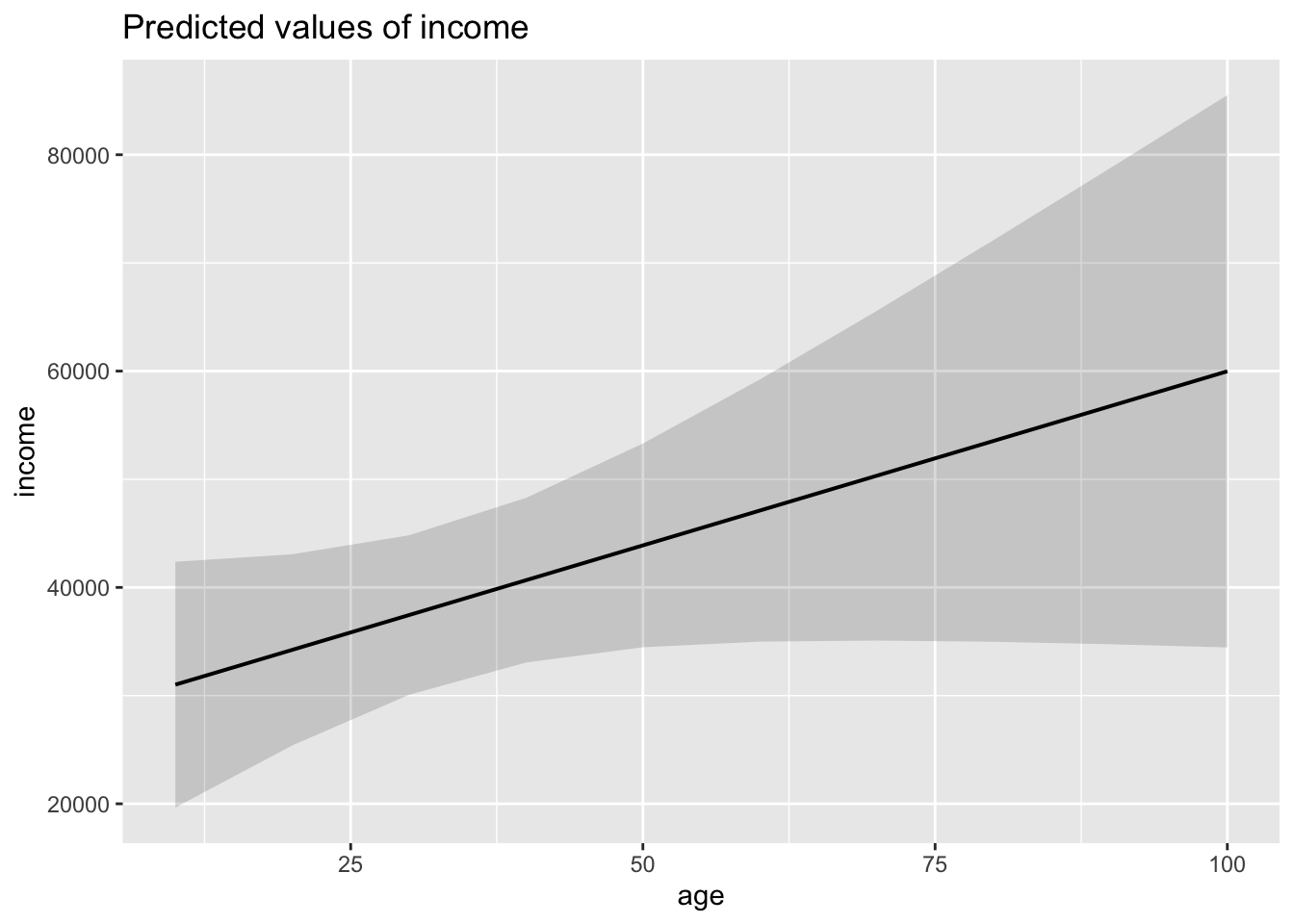
Then, add theme() with options to customize the theme:
ggpredict(mod,
          terms = c("age")) |>
  plot(use_theme = F) +
  theme(panel.border = element_rect(),
        panel.grid = element_blank())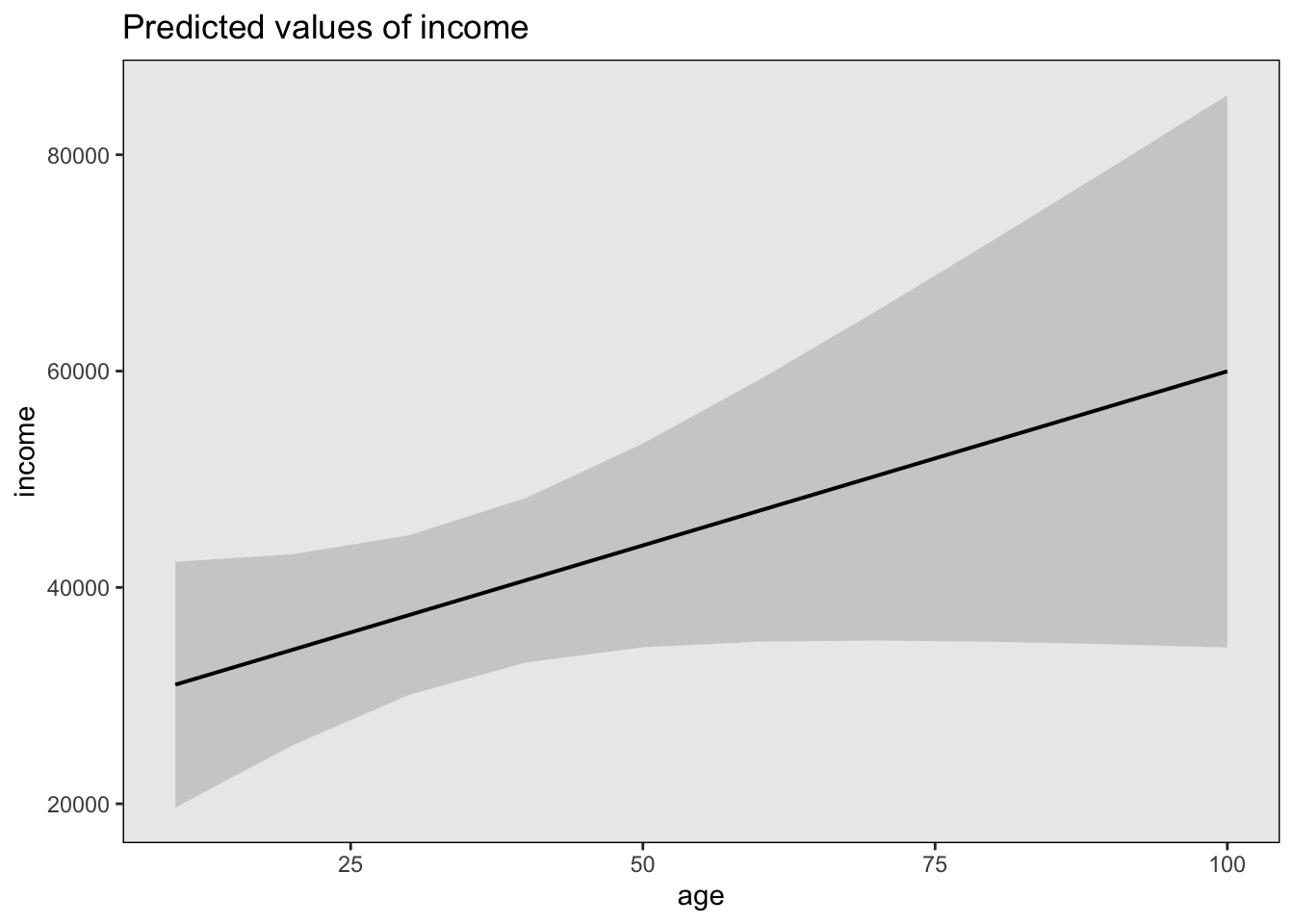
Or use a preset theme:
ggpredict(mod,
          terms = c("age")) |>
  plot(use_theme = F) +
  theme_bw()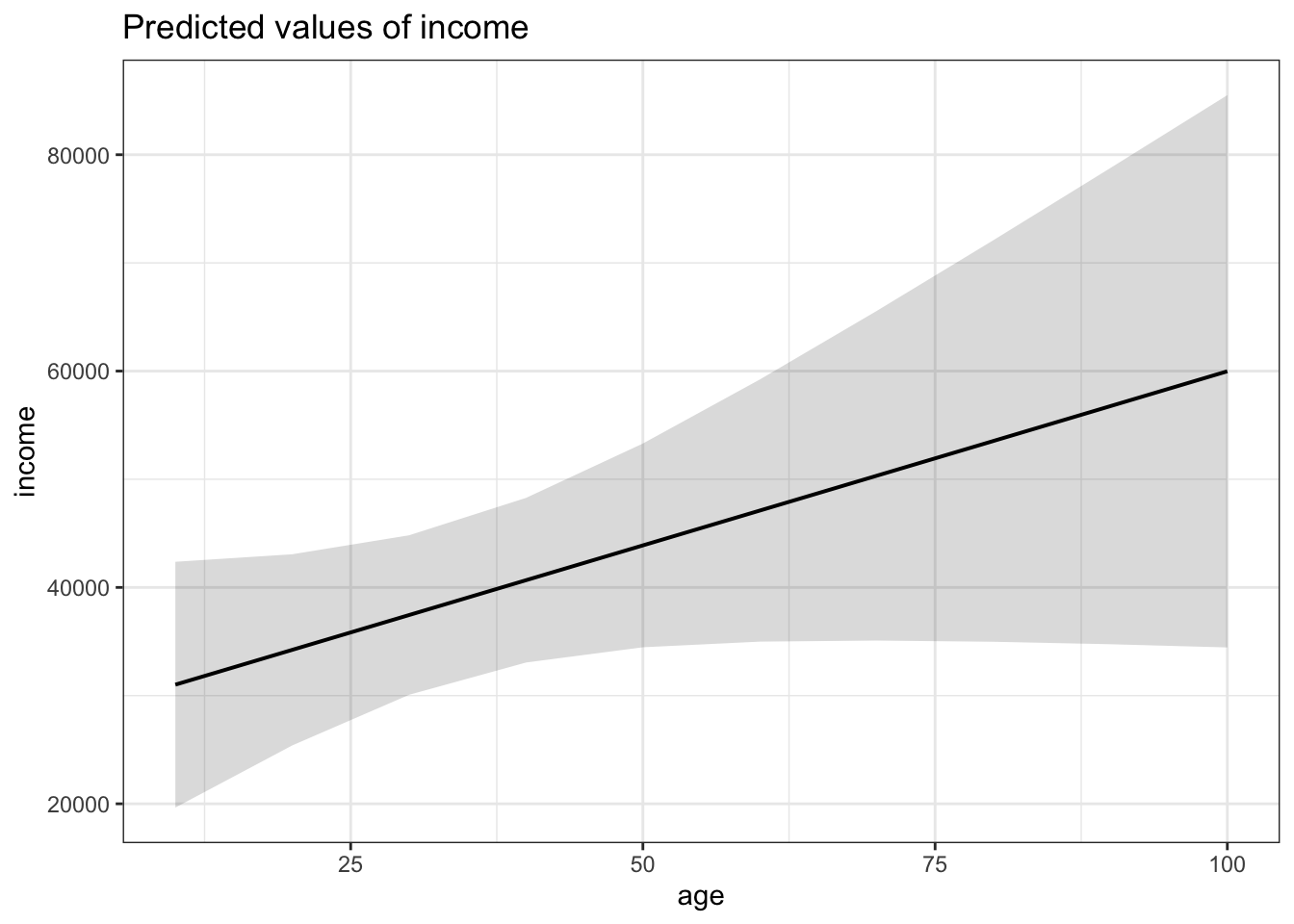
7.3.5 Labels
7.3.5.1 Titles and axes
Labels can be modified with labs(), as with any other ggplot plot.
Remove an existing label by setting it to NULL. To remove the included title, set title = NULL:
ggpredict(mod, terms = c("age", "sex")) |>
  plot() +
  labs(title = NULL,
       x = "Age",
       y = "Income (in US dollars)")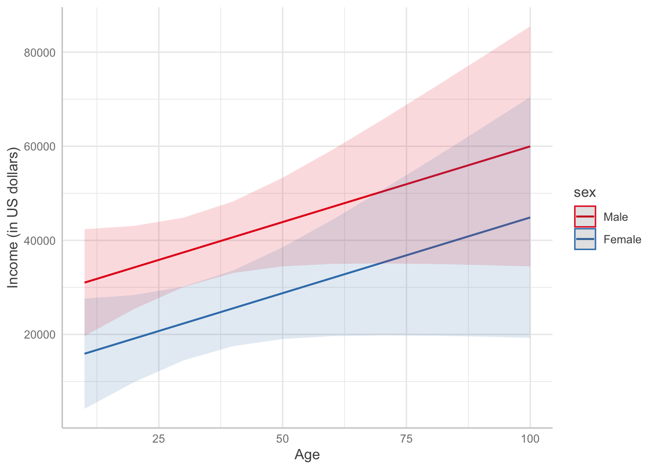
The figure caption text within the manuscript should note the values at which the other variables are held constant: “For individuals with less than high school education working 40 hours per week.”
7.3.5.2 Legend titles
Legends are trickier to modify because a legend’s corresponding aesthetic depends on the colors and variable types.
By default, group is mapped to color, so changing the label for color changes the legend title.
ggpredict(mod,
          terms = c("age", "education")) |>
  plot() +
  labs(color = "Education")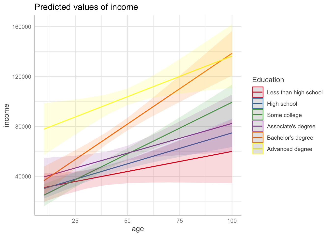
If you create a black-and-white plot (colors = "bw") with a continuous x variable, however, group uses linetype, so the linetype label must be adjusted.
ggpredict(mod,
          terms = c("age", "education")) |>
  plot(colors = "bw") +
  labs(linetype = "Education")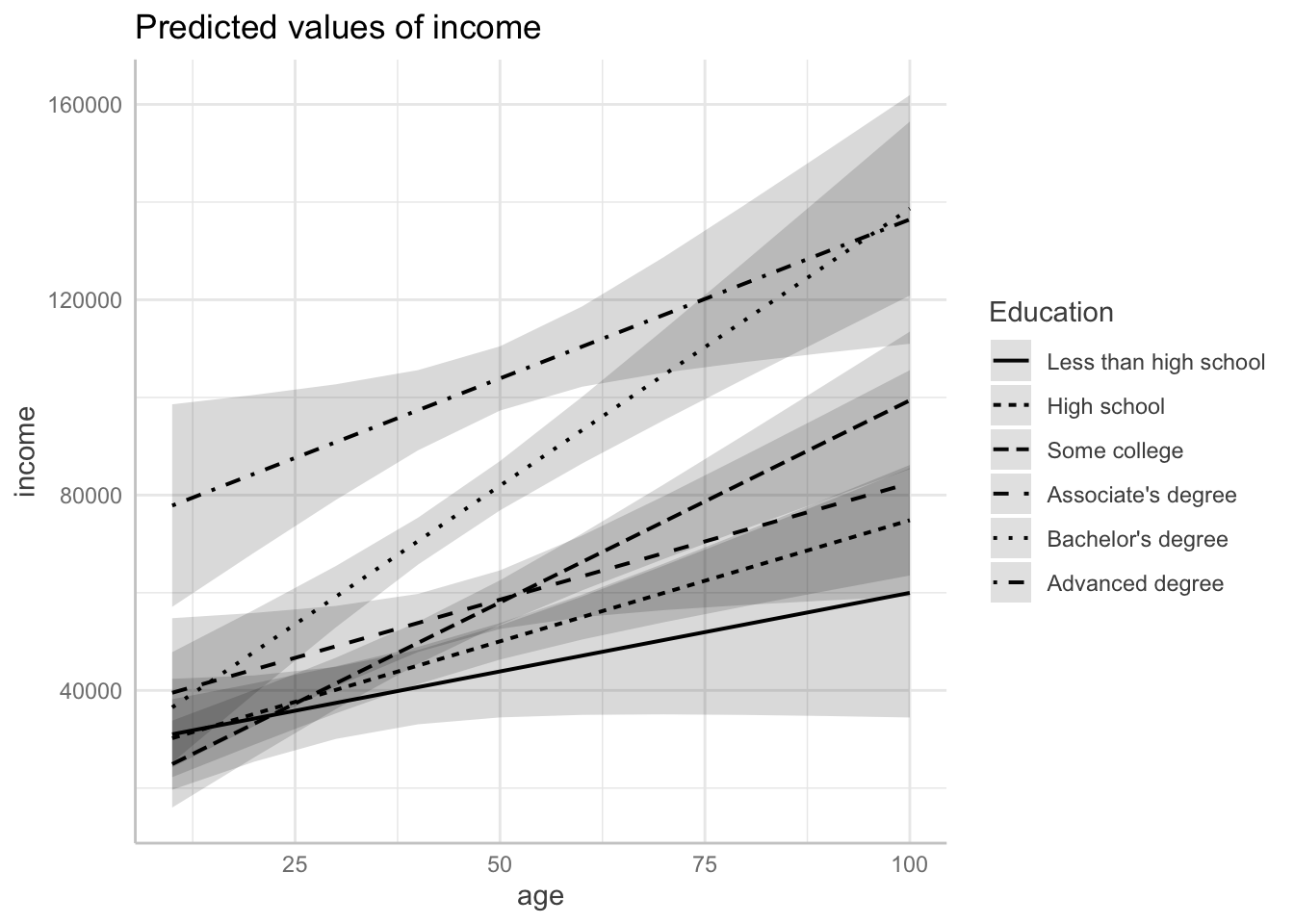
And if you create a black-and-white plot with a categorical x variable, the shape aesthetic is used for group.
ggpredict(mod,
          terms = c("education", "sex")) |>
  plot(colors = "bw") +
  labs(shape = "Sex")
Ignoring unknown labels:
• linetype : "sex"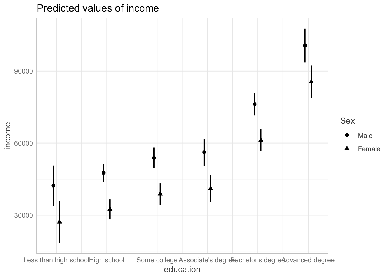
7.3.5.3 Legend labels
To change the level labels in the legend, use a factor wrangling function before passing the ggpredict() result to plot(). The group data is in the group column, so recode it with the pattern:
mutate(group = fct_recode(group,
                          "new_name1" = "old_name1",
"new_name2" = "old_name2"))ggpredict(mod,
terms = c("age", "sex")) |>
mutate(group = fct_recode(group, "M" = "Male", "F" = "Female")) |>
plot() +
labs(color = "Sex")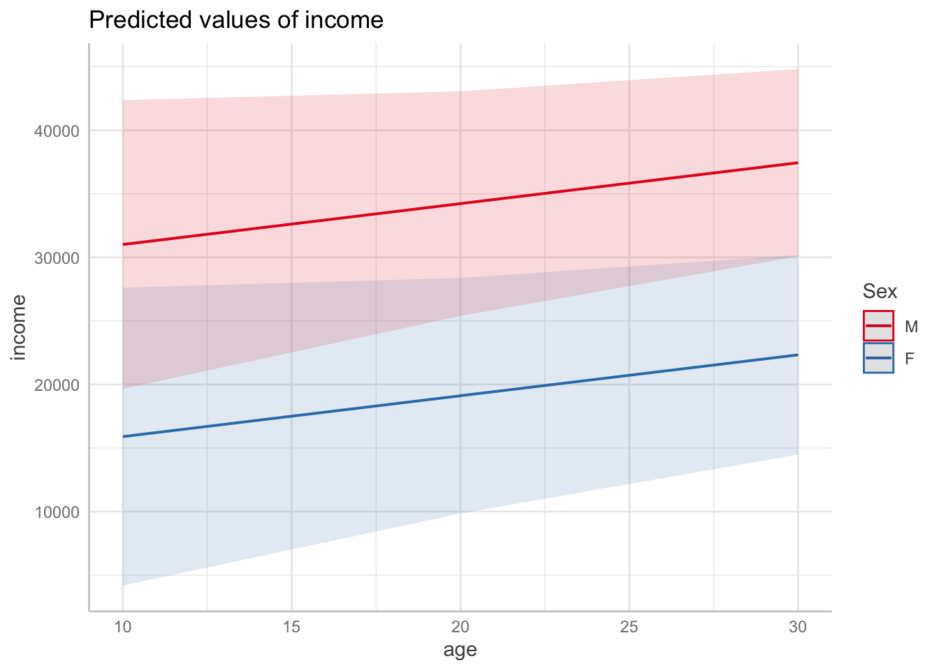
7.4 Interactions
Margins plots are especially useful when we have an interaction term with at least one categorical variable.
The coefficient estimates in interactions with categorical variables are adjustments to the main effects.
The utility of plotting models with interactions is that these plots can tell us where we might or might not see differences, and they can guide our modeling process by helping us decide how to relevel our categorical variables.
This section assumes you are familiar with releveling categorical variables. Learn more in the chapter on categorical variables in Data Wrangling with R.
7.4.1 Categorical x continuous
Fit a model predicting income from sex, age, and their interaction.
mod <- lm(income ~ sex * age, acs)Plot the predicted values by age and sex.
ggpredict(mod, terms = c("age", "sex")) |>
  plot()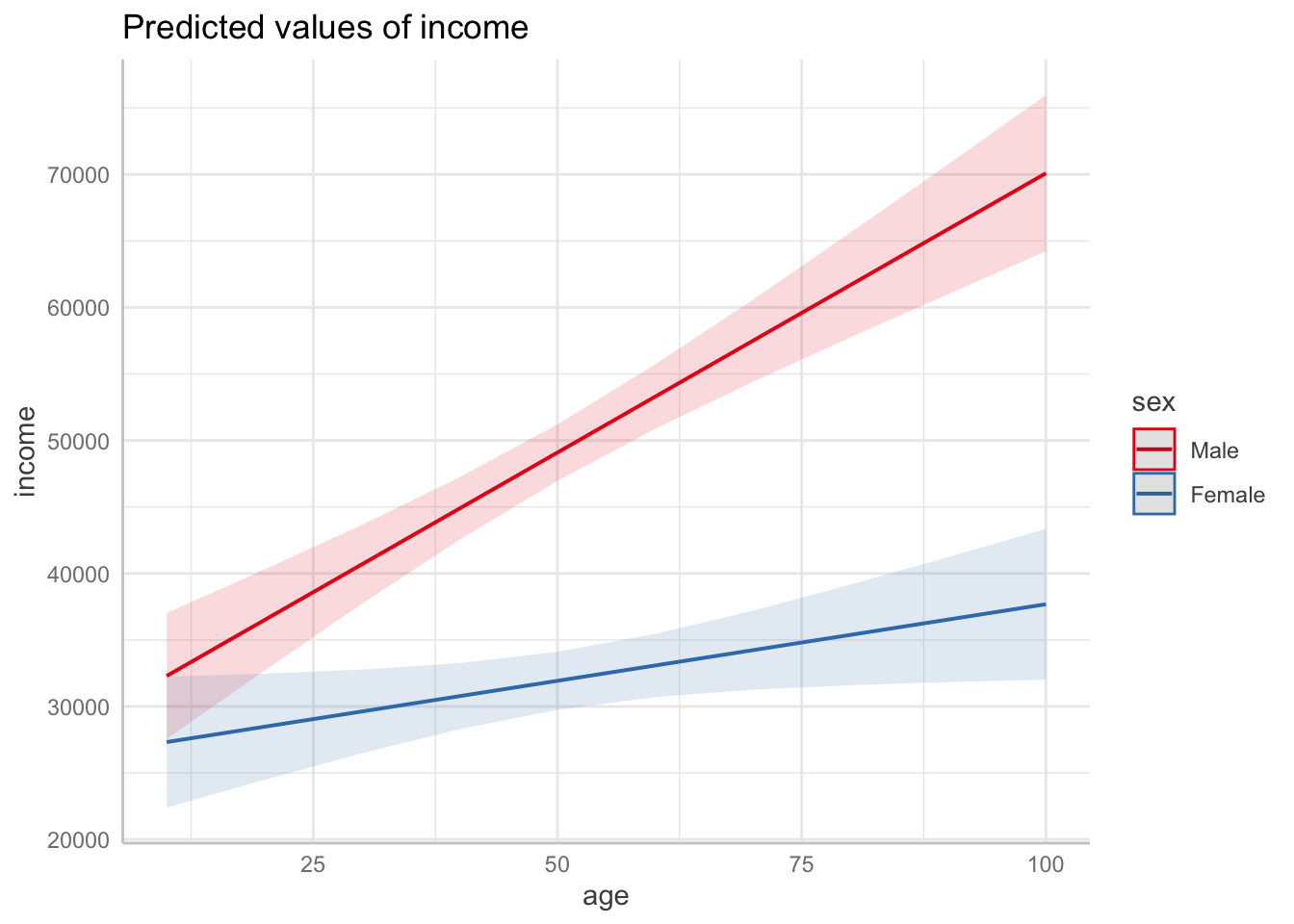
We can see that the slope of age for males is much steeper than the slope for females. We can ask two questions about their slopes:
- Are the slopes statistically significantly different from zero?
- Are the slopes statistically significantly different from each other?
When we have an interaction with a binary variable, the model estimates can only partially answer the first question, though they can help us answer the second question.
The first question can be answered with the coefficient estimate for age. This will tell us whether the slope of age for the reference level of sex is different from zero.
The second question can be answered with the coefficient estimate for the interaction between age and sex. This will tell us whether the slope of age is different between the two levels of sex.
Without releveling, the model estimates cannot tell us whether the slope of the non-reference level of sex (female) is statistically significantly different from zero.
Look at the model estimates. Note the reference level of sex is male.
summary(mod)
Call:
lm(formula = income ~ sex * age, data = acs)

Residuals:
   Min     1Q Median     3Q    Max
-63968 -27314 -10707  11290 632470

Coefficients:
              Estimate Std. Error t value Pr(>|t|)
(Intercept)   28096.31    2917.48   9.630  < 2e-16 ***
sexFemale     -1922.65    4193.36  -0.458    0.647
age             419.90      55.02   7.632 2.85e-14 ***
sexFemale:age  -304.77      77.60  -3.927 8.73e-05 ***
---
Signif. codes:  0 '***' 0.001 '**' 0.01 '*' 0.05 '.' 0.1 ' ' 1

Residual standard error: 50290 on 4201 degrees of freedom
  (795 observations deleted due to missingness)
Multiple R-squared:  0.04078,   Adjusted R-squared:  0.0401
F-statistic: 59.53 on 3 and 4201 DF,  p-value: < 2.2e-16
These estimates tell us, among other things, that:
- The slope of
ageis estimated as 419.9, and it is statistically significant with p < .001. - The slope of
agefor females is estimated to be -304.77 different from the slope ofagefor males, and this difference is statistically significant with p < .001.
What we do not know, however, is whether the slope of age for females is statistically significantly different from zero. If we add together the age slope for males and the interaction of age and sex, we end up with an estimated slope of 115.13. This is closer to zero, but we do not have a significance test until we relevel our sex variable.
We can perform this test by releveling sex to make female the reference category.
(It should be clarified that this is the same model as before. The model fit is exactly the same, just like it would be if we centered or rescaled variables. We only applied a linear transformation to a predictor by shifting its zero point.)
lm(income ~ fct_relevel(sex, "Female") * age, acs) |>
  summary()
Call:
lm(formula = income ~ fct_relevel(sex, "Female") * age, data = acs)

Residuals:
   Min     1Q Median     3Q    Max
-63968 -27314 -10707  11290 632470

Coefficients:
                                   Estimate Std. Error t value Pr(>|t|)
(Intercept)                        26173.67    3012.07   8.690  < 2e-16 ***
fct_relevel(sex, "Female")Male      1922.65    4193.36   0.458   0.6466
age                                  115.13      54.73   2.104   0.0355 *
fct_relevel(sex, "Female")Male:age   304.77      77.60   3.927 8.73e-05 ***
---
Signif. codes:  0 '***' 0.001 '**' 0.01 '*' 0.05 '.' 0.1 ' ' 1

Residual standard error: 50290 on 4201 degrees of freedom
  (795 observations deleted due to missingness)
Multiple R-squared:  0.04078,   Adjusted R-squared:  0.0401
F-statistic: 59.53 on 3 and 4201 DF,  p-value: < 2.2e-16
This formulation of the model tells us that the slope of age for females is statistically significantly different from zero. However, the p-value is just below .05, so we should be suspicious of this finding. Furthermore, we have not even checked our model assumptions!
7.4.2 Categorical x categorical
Now, suppose we want to know about expected differences in income by two categorical variables: sex and level of education. Specifically, we want to investigate the marginal effect of high school education versus some college education for males and females.
Fit a model predicting income from sex, education, and their interaction.
mod <- lm(income ~ sex * education, acs)Plot the predicted values of income by sex and education.
ggpredict(mod,
          terms = c("sex", "education")) |>
  plot()
Ignoring unknown labels:
• linetype : "education"
• shape : "education"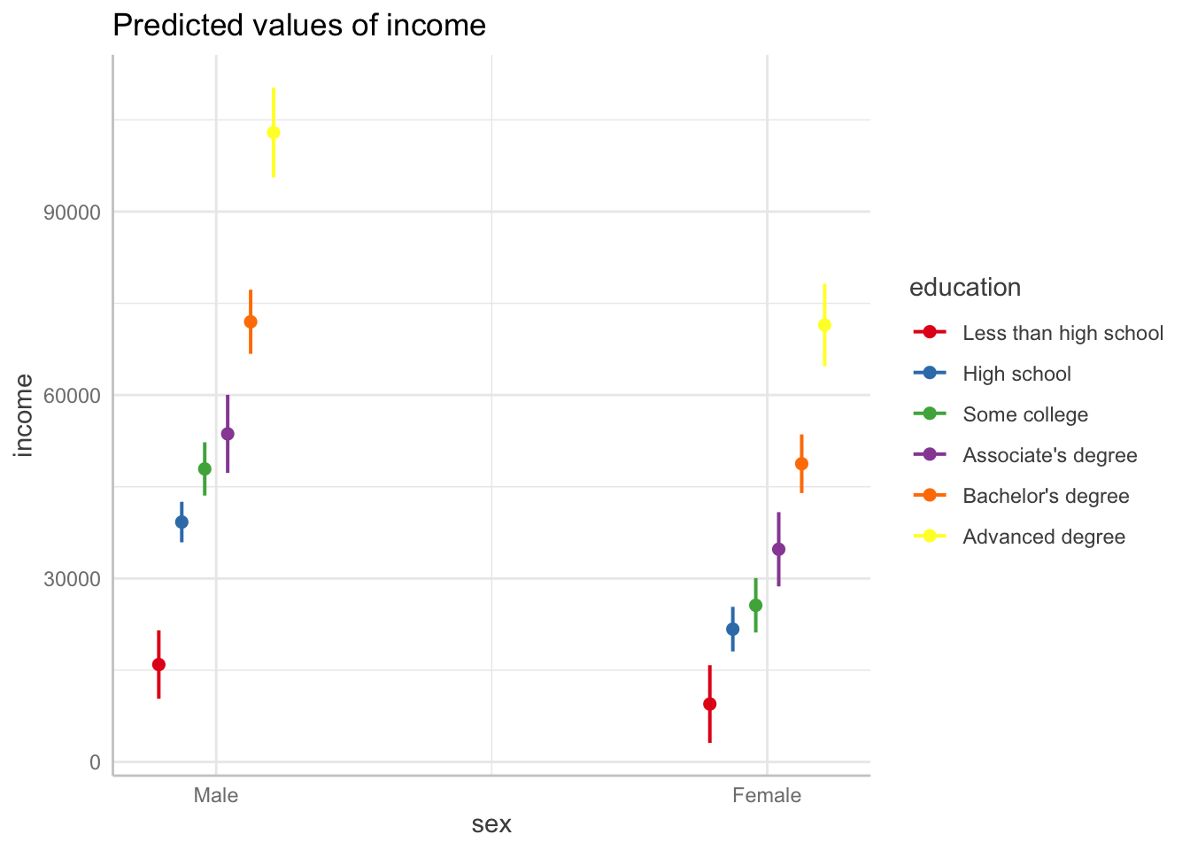
We can see that for males, the expected difference in income between high school education and some college education is statistically significant. Looking at the confidence intervals for these two levels of education (shown as green and blue in the plot), we see that the confidence interval for one level of education does not include the point estimate for the other level of education.
For females, however, we see that these two points have much closer predicted probabilities, and the confidence interval for either one includes the point of the other.
We can formally test these differences by releveling our predictors.
First, test the difference between the two levels of education for males. Leave sex at its reference level (male), but change the reference level for education to high school.
lm(income ~ sex * fct_relevel(education, "High school"), acs) |>
  summary()
Call:
lm(formula = income ~ sex * fct_relevel(education, "High school"),
    data = acs)

Residuals:
   Min     1Q Median     3Q    Max
-98731 -20717  -7448  11083 585769

Coefficients:
                                                                     Estimate
(Intercept)                                                             39227
sexFemale                                                              -17512
fct_relevel(education, "High school")Less than high school             -23304
fct_relevel(education, "High school")Some college                        8689
fct_relevel(education, "High school")Associate's degree                 14421
fct_relevel(education, "High school")Bachelor's degree                  32752
fct_relevel(education, "High school")Advanced degree                    63704
sexFemale:fct_relevel(education, "High school")Less than high school    11060
sexFemale:fct_relevel(education, "High school")Some college             -4793
sexFemale:fct_relevel(education, "High school")Associate's degree       -1358
sexFemale:fct_relevel(education, "High school")Bachelor's degree        -5702
sexFemale:fct_relevel(education, "High school")Advanced degree         -13964
                                                                     Std. Error
(Intercept)                                                                1690
sexFemale                                                                  2514
fct_relevel(education, "High school")Less than high school                 3315
fct_relevel(education, "High school")Some college                          2791
fct_relevel(education, "High school")Associate's degree                    3670
fct_relevel(education, "High school")Bachelor's degree                     3164
fct_relevel(education, "High school")Advanced degree                       4115
sexFemale:fct_relevel(education, "High school")Less than high school       4996
sexFemale:fct_relevel(education, "High school")Some college                4049
sexFemale:fct_relevel(education, "High school")Associate's degree          5150
sexFemale:fct_relevel(education, "High school")Bachelor's degree           4411
sexFemale:fct_relevel(education, "High school")Advanced degree             5680
                                                                     t value
(Intercept)                                                           23.213
sexFemale                                                             -6.966
fct_relevel(education, "High school")Less than high school            -7.030
fct_relevel(education, "High school")Some college                      3.113
fct_relevel(education, "High school")Associate's degree                3.930
fct_relevel(education, "High school")Bachelor's degree                10.352
fct_relevel(education, "High school")Advanced degree                  15.481
sexFemale:fct_relevel(education, "High school")Less than high school   2.214
sexFemale:fct_relevel(education, "High school")Some college           -1.184
sexFemale:fct_relevel(education, "High school")Associate's degree     -0.264
sexFemale:fct_relevel(education, "High school")Bachelor's degree      -1.293
sexFemale:fct_relevel(education, "High school")Advanced degree        -2.458
                                                                     Pr(>|t|)
(Intercept)                                                           < 2e-16
sexFemale                                                            3.77e-12
fct_relevel(education, "High school")Less than high school           2.40e-12
fct_relevel(education, "High school")Some college                     0.00186
fct_relevel(education, "High school")Associate's degree              8.63e-05
fct_relevel(education, "High school")Bachelor's degree                < 2e-16
fct_relevel(education, "High school")Advanced degree                  < 2e-16
sexFemale:fct_relevel(education, "High school")Less than high school  0.02691
sexFemale:fct_relevel(education, "High school")Some college           0.23666
sexFemale:fct_relevel(education, "High school")Associate's degree     0.79203
sexFemale:fct_relevel(education, "High school")Bachelor's degree      0.19620
sexFemale:fct_relevel(education, "High school")Advanced degree        0.01400

(Intercept)                                                          ***
sexFemale                                                            ***
fct_relevel(education, "High school")Less than high school           ***
fct_relevel(education, "High school")Some college                    **
fct_relevel(education, "High school")Associate's degree              ***
fct_relevel(education, "High school")Bachelor's degree               ***
fct_relevel(education, "High school")Advanced degree                 ***
sexFemale:fct_relevel(education, "High school")Less than high school *
sexFemale:fct_relevel(education, "High school")Some college
sexFemale:fct_relevel(education, "High school")Associate's degree
sexFemale:fct_relevel(education, "High school")Bachelor's degree
sexFemale:fct_relevel(education, "High school")Advanced degree       *
---
Signif. codes:  0 '***' 0.001 '**' 0.01 '*' 0.05 '.' 0.1 ' ' 1

Residual standard error: 46860 on 4193 degrees of freedom
  (795 observations deleted due to missingness)
Multiple R-squared:  0.1685,    Adjusted R-squared:  0.1663
F-statistic: 77.25 on 11 and 4193 DF,  p-value: < 2.2e-16
The coefficient for some college is statistically significant, confirming what we saw in the plot.
Now, also change the reference level for sex.
lm(income ~ fct_relevel(sex, "Female") * fct_relevel(education, "High school"), acs) |>
  summary()
Call:
lm(formula = income ~ fct_relevel(sex, "Female") * fct_relevel(education,
    "High school"), data = acs)

Residuals:
   Min     1Q Median     3Q    Max
-98731 -20717  -7448  11083 585769

Coefficients:
                                                                                          Estimate
(Intercept)                                                                                  21715
fct_relevel(sex, "Female")Male                                                               17512
fct_relevel(education, "High school")Less than high school                                  -12244
fct_relevel(education, "High school")Some college                                             3897
fct_relevel(education, "High school")Associate's degree                                      13063
fct_relevel(education, "High school")Bachelor's degree                                       27050
fct_relevel(education, "High school")Advanced degree                                         49740
fct_relevel(sex, "Female")Male:fct_relevel(education, "High school")Less than high school   -11060
fct_relevel(sex, "Female")Male:fct_relevel(education, "High school")Some college              4793
fct_relevel(sex, "Female")Male:fct_relevel(education, "High school")Associate's degree        1358
fct_relevel(sex, "Female")Male:fct_relevel(education, "High school")Bachelor's degree         5702
fct_relevel(sex, "Female")Male:fct_relevel(education, "High school")Advanced degree          13964
                                                                                          Std. Error
(Intercept)                                                                                     1861
fct_relevel(sex, "Female")Male                                                                  2514
fct_relevel(education, "High school")Less than high school                                      3738
fct_relevel(education, "High school")Some college                                               2934
fct_relevel(education, "High school")Associate's degree                                         3613
fct_relevel(education, "High school")Bachelor's degree                                          3074
fct_relevel(education, "High school")Advanced degree                                            3916
fct_relevel(sex, "Female")Male:fct_relevel(education, "High school")Less than high school       4996
fct_relevel(sex, "Female")Male:fct_relevel(education, "High school")Some college                4049
fct_relevel(sex, "Female")Male:fct_relevel(education, "High school")Associate's degree          5150
fct_relevel(sex, "Female")Male:fct_relevel(education, "High school")Bachelor's degree           4411
fct_relevel(sex, "Female")Male:fct_relevel(education, "High school")Advanced degree             5680
                                                                                          t value
(Intercept)                                                                                11.668
fct_relevel(sex, "Female")Male                                                              6.966
fct_relevel(education, "High school")Less than high school                                 -3.276
fct_relevel(education, "High school")Some college                                           1.328
fct_relevel(education, "High school")Associate's degree                                     3.616
fct_relevel(education, "High school")Bachelor's degree                                      8.801
fct_relevel(education, "High school")Advanced degree                                       12.702
fct_relevel(sex, "Female")Male:fct_relevel(education, "High school")Less than high school  -2.214
fct_relevel(sex, "Female")Male:fct_relevel(education, "High school")Some college            1.184
fct_relevel(sex, "Female")Male:fct_relevel(education, "High school")Associate's degree      0.264
fct_relevel(sex, "Female")Male:fct_relevel(education, "High school")Bachelor's degree       1.293
fct_relevel(sex, "Female")Male:fct_relevel(education, "High school")Advanced degree         2.458
                                                                                          Pr(>|t|)
(Intercept)                                                                                < 2e-16
fct_relevel(sex, "Female")Male                                                            3.77e-12
fct_relevel(education, "High school")Less than high school                                0.001062
fct_relevel(education, "High school")Some college                                         0.184179
fct_relevel(education, "High school")Associate's degree                                   0.000303
fct_relevel(education, "High school")Bachelor's degree                                     < 2e-16
fct_relevel(education, "High school")Advanced degree                                       < 2e-16
fct_relevel(sex, "Female")Male:fct_relevel(education, "High school")Less than high school 0.026906
fct_relevel(sex, "Female")Male:fct_relevel(education, "High school")Some college          0.236657
fct_relevel(sex, "Female")Male:fct_relevel(education, "High school")Associate's degree    0.792026
fct_relevel(sex, "Female")Male:fct_relevel(education, "High school")Bachelor's degree     0.196195
fct_relevel(sex, "Female")Male:fct_relevel(education, "High school")Advanced degree       0.014004

(Intercept)                                                                               ***
fct_relevel(sex, "Female")Male                                                            ***
fct_relevel(education, "High school")Less than high school                                **
fct_relevel(education, "High school")Some college
fct_relevel(education, "High school")Associate's degree                                   ***
fct_relevel(education, "High school")Bachelor's degree                                    ***
fct_relevel(education, "High school")Advanced degree                                      ***
fct_relevel(sex, "Female")Male:fct_relevel(education, "High school")Less than high school *
fct_relevel(sex, "Female")Male:fct_relevel(education, "High school")Some college
fct_relevel(sex, "Female")Male:fct_relevel(education, "High school")Associate's degree
fct_relevel(sex, "Female")Male:fct_relevel(education, "High school")Bachelor's degree
fct_relevel(sex, "Female")Male:fct_relevel(education, "High school")Advanced degree       *
---
Signif. codes:  0 '***' 0.001 '**' 0.01 '*' 0.05 '.' 0.1 ' ' 1

Residual standard error: 46860 on 4193 degrees of freedom
  (795 observations deleted due to missingness)
Multiple R-squared:  0.1685,    Adjusted R-squared:  0.1663
F-statistic: 77.25 on 11 and 4193 DF,  p-value: < 2.2e-16
For females, the coefficient estimate for some college is not statistically significant at p = .18, again confirming what we saw in the plot.
This approach of first examining margins plots helps guide our modeling, and it prevents us from making incorrect inferences about effects across the levels of categorical variables. If we did not visualize the results and relevel sex, we may have incorrectly assumed that there was a significant difference between two levels of education, but in fact this was only true for males and not females!
7.5 Logistic regression
The examples on this page so far have all used linear regression, but ggpredict() can help us visualize results from many kinds of models, including logistic regression.
As an example, we can first add a binary variable indicating whether somebody has a higher education degree, and then fit a model predicting this variable.
acs <-
  acs |>
  mutate(higher_ed_degree = as.numeric(education %in% c("Bachelor's degree", "Advanced degree")))

mod <-
  glm(higher_ed_degree ~ age * sex + commute_time + weeks_worked + hours_worked,
      acs,
      family = binomial)
Neither the ggpredict() nor the plot() functions need anything special. We can continue to use them just as we did for linear regression. ggpredict() will calculate the predicted probabilities associated with the terms we provided.
ggpredict(mod, terms = c("age", "sex")) |>
  plot()
Data were 'prettified'. Consider using `terms="age [all]"` to get smooth
plots.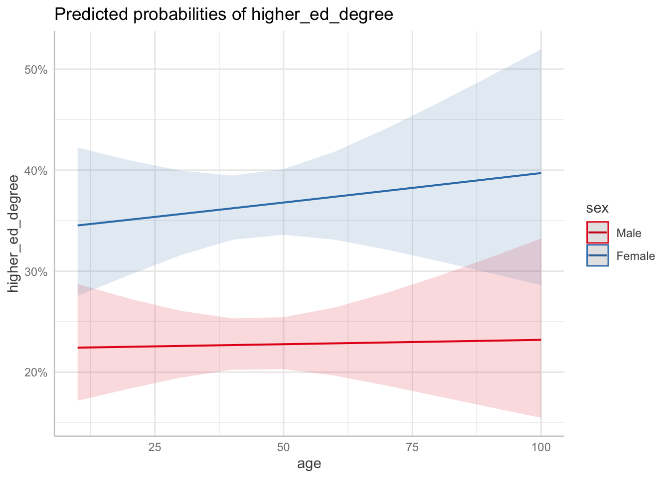
7.6 Saving plots
Use ggsave() to save plots. This function saves the most recently created plot, and it supports several file extensions. See the chapter on Saving Plots for more on ggsave().
ggsave("plot.png", width = 6, height = 4)7.7 Exercises
Continue to use the ACS dataset, or pick one of the following datasets from the tidyverse:
msleep, mammals’ sleep statistics and other characteristicsstarwars, attributes of Star Wars charactersdiamonds, attributes of diamondsmidwest, data on Midwest counties from the 2000 Census
Fit a model with at least three predictors. Do not concern yourself with whether the model makes sense or violates assumptions.
Create two margins plots, where one has at least two terms.
Plot margins at specific values of your terms.
Plot margins under custom constraints on the covariates.
Change the colors of your plot to be black and white.
Change the labels of the axes and legend.
Move or remove the legend.
Save your plot.