| Complete Data | Listwise Deletion | |||||
| Parameter | Estimate | SE | CI | Estimate | SE | CI |
| Intercept | -0.02 | 0.03 | -0.08 – 0.04 | -0.02 | 0.03 | -0.08 – 0.04 |
| x1 | 0.96 | 0.03 | 0.90 – 1.03 | 0.97 | 0.03 | 0.90 – 1.03 |
| x2 | 1.01 | 0.03 | 0.95 – 1.07 | 1.01 | 0.03 | 0.94 – 1.07 |
| Observations | 1000 | 912 | ||||
4 Regression
The files for this page’s example analysis are
01_regression.R: the R script that simulates the data and fits frequentist models01_regression.csv: the data file01_regression.imp: the Blimp script01_regression.blimp-out: the Blimp output file
All files are available at this link.
The following issues are discussed:
- Number of MCMC iterations
- Random seed selection
- Regression
- Missing data mechanisms: MCAR
- Convergence
- Mixing and stationarity
- Potential scale reduction (PSR) factors
- Number of effective samples
- How to improve fit
4.1 Example Model
The dataset for this example has 1000 observations. 8.8% of x1 is missing. x1 is missing completely at random (MCAR); its missingness is unrelated to any observed or unobserved values.
Below is a table of estimates from a model predicting y with (1) the complete data and (2) the data after some values in x1 were made missing, using a listwise deletion procedure.
As expected, under MCAR, estimates are unbiased.
4.2 Blimp Input
The Blimp script for this analysis is as follows:
DATA: 01_regression.csv;
FIXED: x2;
MODEL: y ~ x1 x2; # regress y on x1 and x2
SEED: 123;
BURN: 5000;
ITERATIONS: 5000;
Select sections of the script are now discussed.
4.2.1 Basic Syntax
Each line in a Blimp script follows this pattern:
COMMAND: value;The commands are not case-sensitive, but capitalizing them improves readability. Line breaks are ignored, and multiple values can be supplied so long as each ends with a semicolon (e.g., multiple formulas as in the mediation example:
COMMAND:
value;
COMMAND:
value;
value;
Comments are done with the # symbol. Anything after a # on the same line is ignored.
4.2.2 Missing Data
By default, Blimp will only interpret NA as missing. The data file has NA for missing, so nothing needs to be specified.
Any exogenous variables without any missing data can be included after the FIXED command, which we have done here for x2. This speeds up computation since Blimp uses a round-robin technique for imputing predictors, where each predictor is regressed on all the others. Specifying a variable as fully observed via the FIXED command skips the model predicting that variable.
4.2.3 Model Syntax
Regression formulas are specified as
outcome ~ predictor1 predictor2;where the anything to the left of ~ is an outcome, and anything to the right is a predictor.
4.2.4 Random Seeds
Blimp requires a random seed. Doing so ensures that the results are the same each time we run the script, as long as nothing else has changed. Any number can be used as a random seed: 123 (if you’re not feeling creative), 1, your zip code, today’s date, your birthday, your favorite number, etc.
4.2.5 Iterations
We must also specify the number of burn-in (BURN) and post-burn-in iterations (ITERATIONS).
MCMC chains start at random values for each parameter, and we discard early iterations to remove the effect of their starting values. This period is called the burn-in or “warm-up.”1 We then keep the post-burn-in iterations to get a posterior distribution. The default number of chains is two, which is sufficient but can be modified with the CHAINS command. Each chain discards BURN iterations, and then ITERATIONS is split among the chains. Each chain, therefore, has a total number of iterations of \(BURN + \frac{ITERATIONS}{Number\: of\: chains}\). In our example with 5000 for each command, each chain completes 7500 iterations, of which we only keep the last 2500.
As a starting point, you may try starting with 5000 burn-in and post-burn-in iterations, and then add to that depending on convergence.
4.3 Blimp Output
Running the Blimp script produces this output file:
---------------------------------------------------------------------------

                                   Blimp
                                  3.2.10

             Blimp was developed with funding from Institute of
           Education Sciences awards R305D150056 and R305D190002.

            Craig K. Enders, P.I. Email: cenders@psych.ucla.edu
           Brian T. Keller, Co-P.I. Email: btkeller@missouri.edu
                 Han Du, Co-P.I. Email: hdu@psych.ucla.edu
                 Roy Levy, Co-P.I. Email: roy.levy@asu.edu

              Programming and Blimp Studio by Brian T. Keller

                   There is no expressed license given.

---------------------------------------------------------------------------


ALGORITHMIC OPTIONS SPECIFIED:

  Imputation method:                 Fully Bayesian model-based
  MCMC algorithm:                    Full conditional Metropolis sampler with
                                       Auto-Derived Conditional Distributions
  Between-cluster imputation model:  Not applicable, single-level imputation
  Prior for random effect variances: Not applicable, single-level imputation
  Prior for residual variances:      Zero sum of squares, df = -2 (PRIOR2)
  Prior for predictor variances:     Unit sum of squares, df = 2 (XPRIOR1)
  Chain Starting Values:             Random starting values


BURN-IN POTENTIAL SCALE REDUCTION (PSR) OUTPUT:

  NOTE: Split chain PSR is being used. This splits each chain's
        iterations to create twice as many chains.

  Comparing iterations across 2 chains     Highest PSR   Parameter #
                          126 to 250             1.025            10
                          251 to 500             1.014             4
                          376 to 750             1.017            10
                          501 to 1000            1.007             1
                          626 to 1250            1.006             8
                          751 to 1500            1.004            10
                          876 to 1750            1.008            11
                         1001 to 2000            1.002            11
                         1126 to 2250            1.003            11
                         1251 to 2500            1.003            11
                         1376 to 2750            1.001             3
                         1501 to 3000            1.001             7
                         1626 to 3250            1.002             5
                         1751 to 3500            1.002            11
                         1876 to 3750            1.002            11
                         2001 to 4000            1.001            11
                         2126 to 4250            1.002            10
                         2251 to 4500            1.001             5
                         2376 to 4750            1.001             7
                         2501 to 5000            1.001             7


METROPOLIS-HASTINGS ACCEPTANCE RATES:

  Chain 1:

    Variable                            Type    Probability   Target Value
    x1                            imputation          0.499          0.500

  NOTE: Suppressing printing of 1 chains.
        Use keyword 'tuneinfo' in options to override.


DATA INFORMATION:

  Sample Size:              1000
  Missing Data Rates:

                        y = 00.00
                       x1 = 08.80


MODEL INFORMATION:

  NUMBER OF PARAMETERS
    Outcome Models:         4
    Predictor Models:       3

  PREDICTORS
    Fixed variables:        x2
    Incomplete continuous:  x1

  MODELS
    [1]  y ~ Intercept x1 x2


WARNING MESSAGES:

  No warning messages.


MODEL FIT:


  INFORMATION CRITERIA

    Marginal Likelihood
      DIC2                  2797.690
      WAIC                  2814.756

    Conditional Likelihood
      DIC2                  2797.690
      WAIC                  2814.756


CORRELATIONS AMONG RESIDUALS:

  No residual correlations.


OUTCOME MODEL ESTIMATES:

  Summaries based on 5000 iterations using 2 chains.


Outcome Variable:  y

Parameters                           Median     StdDev       2.5%      97.5%        PSR      N_Eff
                                -------------------------------------------------------------------
Variances:
  Residual Var.                       0.938      0.044      0.859      1.029      1.002   3527.214

Coefficients:
  Intercept                          -0.021      0.031     -0.084      0.040      1.001   4155.296
  x1                                  0.964      0.034      0.898      1.031      1.001   3914.456
  x2                                  1.009      0.031      0.951      1.069      1.001   3898.620

Standardized Coefficients:
  x1                                  0.509      0.015      0.479      0.538      1.002   3884.470
  x2                                  0.572      0.014      0.543      0.599      1.001   3662.815

Proportion Variance Explained
  by Coefficients                     0.721      0.013      0.696      0.744      1.003   3567.152
  by Residual Variation               0.279      0.013      0.256      0.304      1.003   3567.152

                                -------------------------------------------------------------------


PREDICTOR MODEL ESTIMATES:

  Summaries based on 5000 iterations using 2 chains.


Missing predictor:  x1

Parameters                           Median     StdDev       2.5%      97.5%        PSR      N_Eff
                                -------------------------------------------------------------------

Grand Mean                           -0.013      0.031     -0.072      0.049      1.000   4300.645

Level 1:
  x2                                  0.216      0.029      0.159      0.273      1.001   3883.537
  Residual Var.                       0.888      0.041      0.812      0.974      1.000   3451.772

                                -------------------------------------------------------------------
Select sections of the output are now discussed.
4.3.1 Outcome Models
First off, how well did our model recover the true values? The Outcome Variable: y section contains a table of estimates. For each parameter, we get a measure of central tendency (median) and measures of spread (SD and 95% credible interval upper and lower limits). We also get PSR and N_Eff statistics; see the next section on convergence.
The intercept was simulated to be about zero, and the coefficients of x1 and x2 to be about one. These values are close to the parameter medians and well within their credible intervals. We would conclude that there is a 95% probability that the true effect of x1 on y is between 0.898 and 1.031.
Importantly, our model used all 1000 observations, even though x1 had missing values. At each iteration, plausible values for x1 were imputed, the focal model was estimated, estimates were saved, new values were imputed, and so on. Just like that, with such simple syntax, we fit a Bayesian regression model to incomplete data!
4.3.2 Convergence
How do we know if our model converged? What is convergence, exactly?
Summary:
- If the potential scale reduction factor for any parameter is more than 1.05, increase the burn-in iterations.
- If the number of effective samples for any parameter is less than 100, increase the post-burn-in iterations.
- If convergence issues persist, revise the model.
4.3.2.1 Mixing and Stationarity
We say that a model has converged if its MCMC chains are mixed and stationary. Mixing means that the chains are exploring the same parameter space (i.e., looking around the same values), and stationarity means the chains have settled in that parameter space (i.e., not wandering around).
It will be helpful to see what different combinations of mixed and not-mixed, stationary and not-stationary look like:
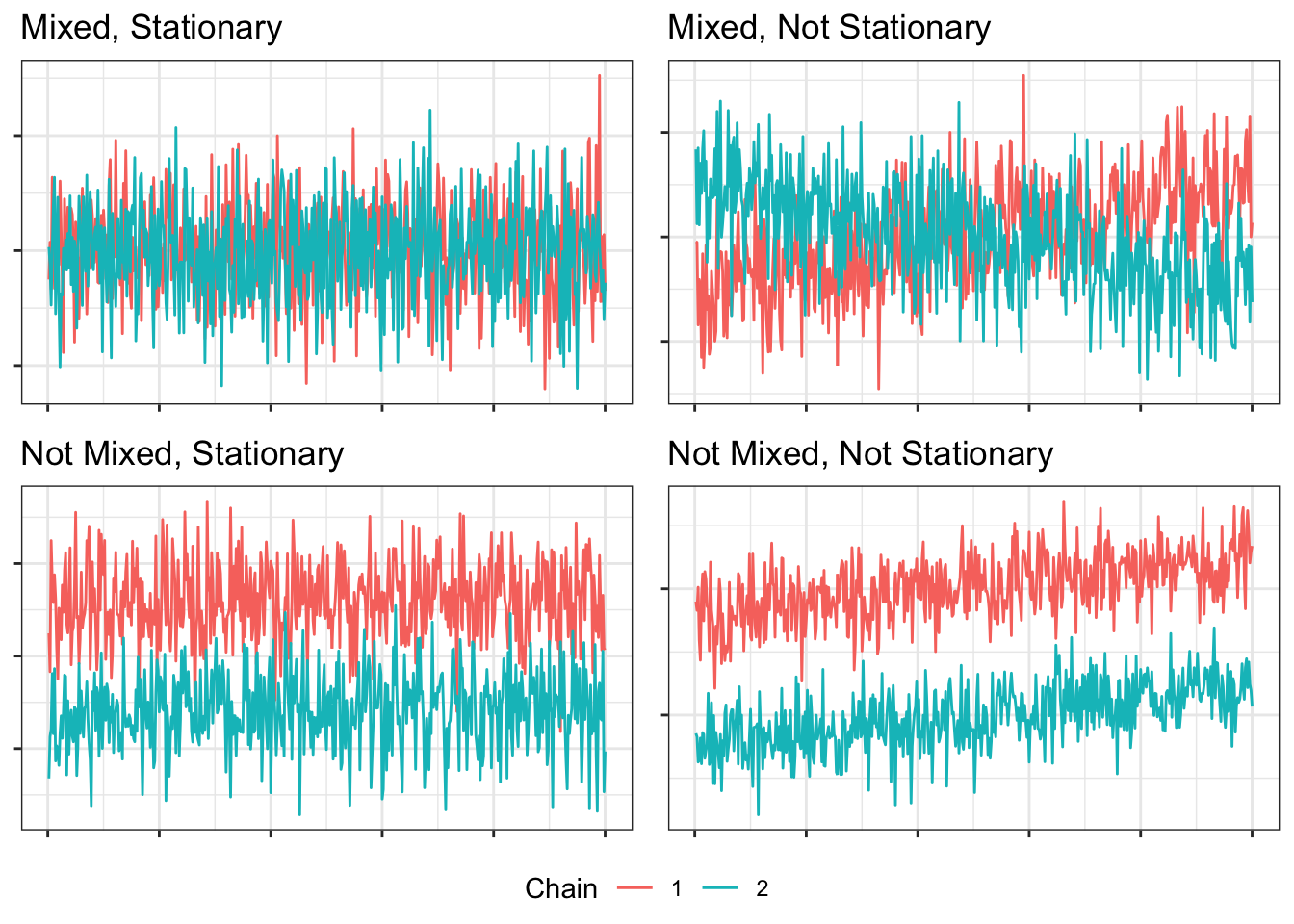
These examples are simulated to be clear-cut, but real trace plots from real models with real data are less clear.
Inspection of [trace] plots is a notoriously unreliable method of assessing convergence and in addition is unwieldy when monitoring a large number of quantities of interest.2
Instead, we can use potential scale reduction (PSR) factors.
4.3.2.2 Potential Scale Reduction
PSRs are essentially a weighted combination of total variance divided by the within-chain variance. Each chain is split in two so that we get twice as many half-chains as chains. The PSR’s minimum is 1, where there is no between-chain variance. A low PSR indicates that we have achieved both mixing and stationarity. Less mixing would mean greater between-chain variance, and less stationarity would mean greater variance between a single chain’s two halves. Either of these would increase the numerator in the calculation of the PSR, meaning the PSR is a sufficient convergence diagnostic statistic.
The practical meaning of the PSR is indicated by its name; it is an estimate for how much a parameter’s posterior variance would decrease if the chain could continue forever. In other words, would we get a more accurate posterior distribution if we let the chains run longer?
The beginning of the Blimp output describes the PSRs for the burn-in period. The MCMC chains are taken in small pieces, and the greatest PSR is reported along with which parameter it belonged to. The identity of these parameters can be found by adding to our script:
OPTIONS: labels;Further down in the output, each parameter’s PSR is reported for the post-burn-in iterations.
What we want to see is that all PSRs are below 1.05 by the end of the burn-in period. If not, increase the number of burn-in iterations to allow the chains to find and settle in a common posterior distribution.
4.3.2.3 Number of Effective Samples
Another convergence diagnostic is the number of effective samples. This is found in the rightmost column of the tables of parameter estimates, N_Eff. Iterations in MCMC chains are necessarily autocorrelated, and the effective sample size is an estimate of the sample size for that parameter after correcting for dependence. In order to get an unbiased estimate of the posterior variance, we want N_Eff to be at least 100. If it is under that, increase the number of post-burn-in iterations.
4.3.2.4 Continuing Convergence Issues
If the PSRs and/or numbers of effective samples do not meet their cutoffs (PSR < 1.05; N_Eff ≥ 100) after increasing the numbers of iterations to many tens of thousands or hundreds of thousands, revisit the model form. You may need to simplify the model (e.g., drop predictors from focal model, not estimate auxiliary models, remove random slopes, simplify selection models).
4.3.3 Fit Statistics
The WAIC, a Bayesian analog of the AIC, is reported. These statistics, like the AIC and BIC, are meaningless on their own, but they can be used for model comparison, where lower values indicate better fit.
With unclustered data, the marginal and conditional WAIC will be the same. The marginal WAIC tells us about generalizing to new clusters, and the conditional WAIC to new individuals.3 Model comparisons should take both into account, as changes in fit may show up at either level.4
4.3.4 Predictor Models
Blimp regresses each missing predictor (any predictor not specified after FIXED) on all the other predictors at each iteration, and these model estimates are also returned. Here, x1 was regressed on x2. These models do not need to be interpreted, but they give us insight into the relationships between our predictors, and their estimates informed posterior distributions of our focal model.
4.4 Exercise
Fit a regression model with the dataset exercise_01.csv. (All files are available at this link.) Regress y on x1 and x2. You have reason to believe y is missing completely at random. The coefficients on both predictors should be around 1.
Gelman et al., 2021, p. 282↩︎
Gelman et al., 2021, p. 285↩︎
Merkle, E. C., Furr, D., & Rabe-Hesketh, S. (2019) Bayesian comparison of latent variable models: Conditional versus marginal likelihoods. Psychometrika, 84(3), 802-829. https://doi.org/10.1007/s11336-019-09679-0↩︎
Gelman, A., Vehtari, A., Simpson, D., Margossian, C. C., Carpenter, B. Yao, Y., Kennedy, L., Gabry, J., Bürkner, P.-C., & Modrák, M. (2020). Bayesian workflow. arXiv. https://doi.org/10.48550/arXiv.2011.01808↩︎