![]()
3 Introduction to Blimp
In this section of the book, we will first look at the Blimp modeling framework and user interface. The next few chapters take an example-based approach to demonstrating Blimp’s capabilities; features are introduced in the context of example models. These include model syntax, diagnosing convergence, selection models for missing data, latent variable specification, and random effects.
3.1 Modeling Framework
Blimp is an easy-to-use software program for Bayesian estimation. It can be used for a variety of statistical models, anything from simple regression up to multilevel latent growth models. It is especially useful for missing data analysis due to its unique modeling framework.
Blimp uses a modeling framework called factored regression specification or sequential specification. This framework allows us to model complex multivariate distributions and account for nonnormal relationships among predictors. To learn more, see the section titled “Blimp’s Modeling Framework” in the User’s Guide and its references, or Craig Enders’ video explanation.
3.2 Interface
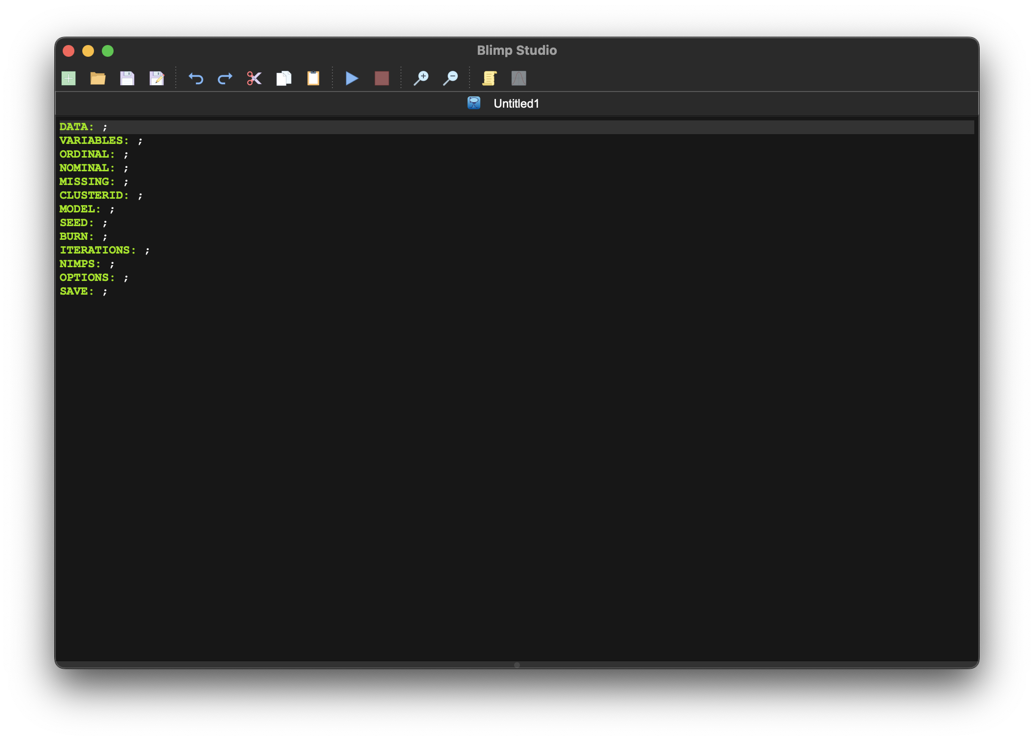
Upon opening Blimp, you will have a blank window:
Click the new script icon  in the top left to open a new script. Some commands are included by default. These can be changed in Preferences > Syntax Window.
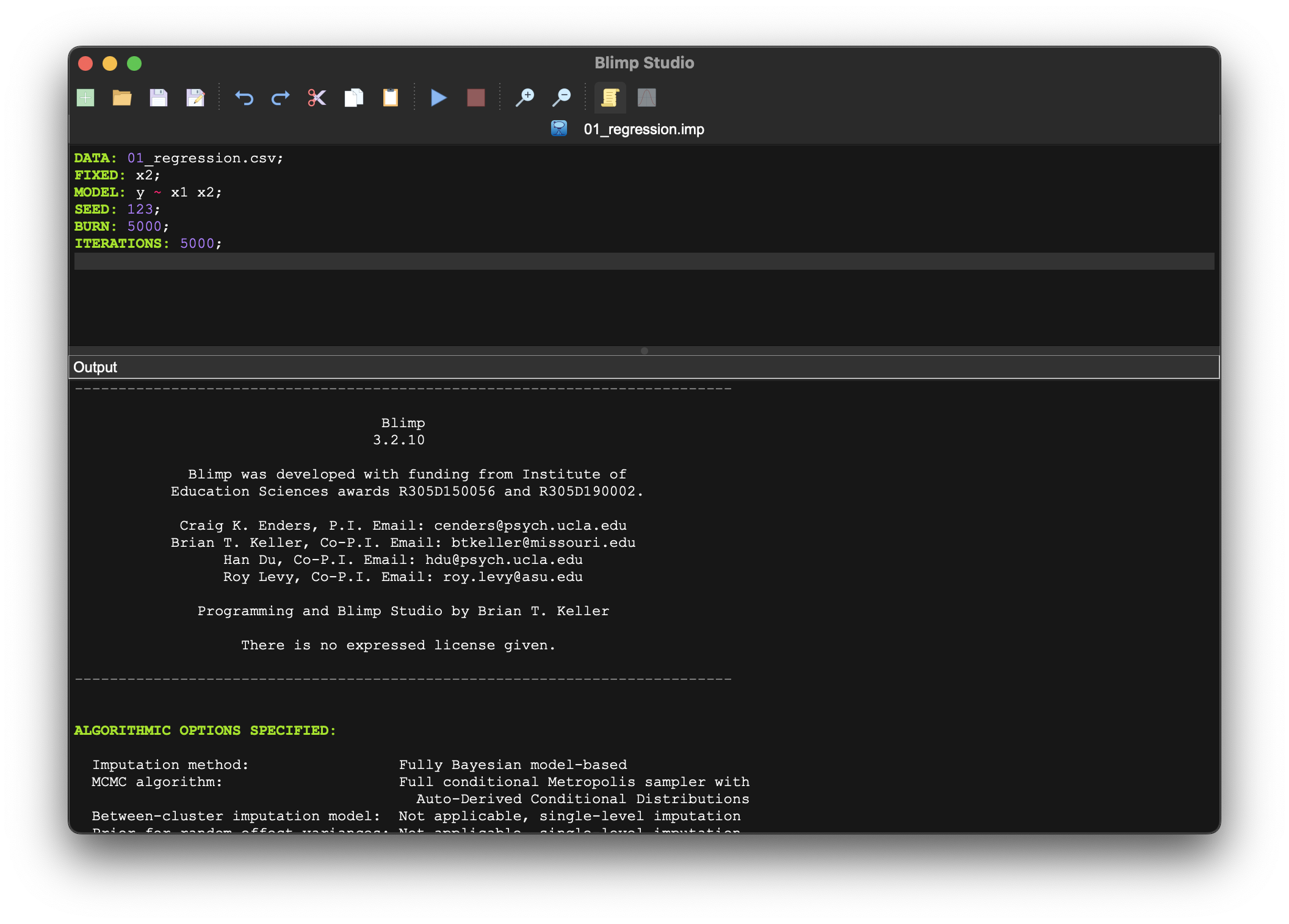
After running a script, an output pane will be revealed.
Plots will also be generated by default. Interpretation of trace plots is subjective, and using potential scale reduction (PSR) factors for diagnosing convergence is preferred, as discussed in Diagnosing Convergence. Disabling plots can also speed up processing; disable them in Preferences > Plot Settings > Default Auto Show Plot.
3.3 Files
You will work with three types of files in Blimp, all of which are plain text files.
.imp- script with model syntax and estimation settings- data - plain text data files like .csv, .dat, or .txt (not binary files like .rds or .dta)
.blimp-out- output with fit information and model estimates
Blimp assumes that the data file is in the same folder as the script, and the output file will be created in that same folder. This is true even if we have multiple scripts open from multiple locations on our computer; each one will look in its own folder.
3.4 Running Blimp at the SSCC
Blimp is available on the SSCC’s Linux servers, so it can be run on Linstat and Slurm. Blimp can be run through the command line with
blimp filename.imp --output filename.blimp-outWhere filename.imp is the name of the input file, and filename.blimp-out is where to save the estimates.
Slurm Assistant can help craft this command for you. See the Guide to Research Computing for more about using Slurm.
More options can be included after the Blimp command, such as the random seed and filepaths for saving estimates. See the “Running From Terminal” section of the User’s Guide.