6 Mediation
The files for this page’s example analysis are
03_mediation.R: the R script that simulates the data and fits frequentist models03_mediation.csv: the data file03_mediation.imp: the Blimp script03_mediation.blimp-out: the Blimp output file
All files are available at this link.
The following issues are discussed:
- Latent variables
- Named models
- Additional parameters
- Missing data mechanisms: MAR
6.1 Example Model
The dataset for this example has 100 observations. 28% of m is missing. m is missing at random (MAR); its missingness is conditional on the values of x, a latent variable created from x1-x5 (but not included in this dataset).
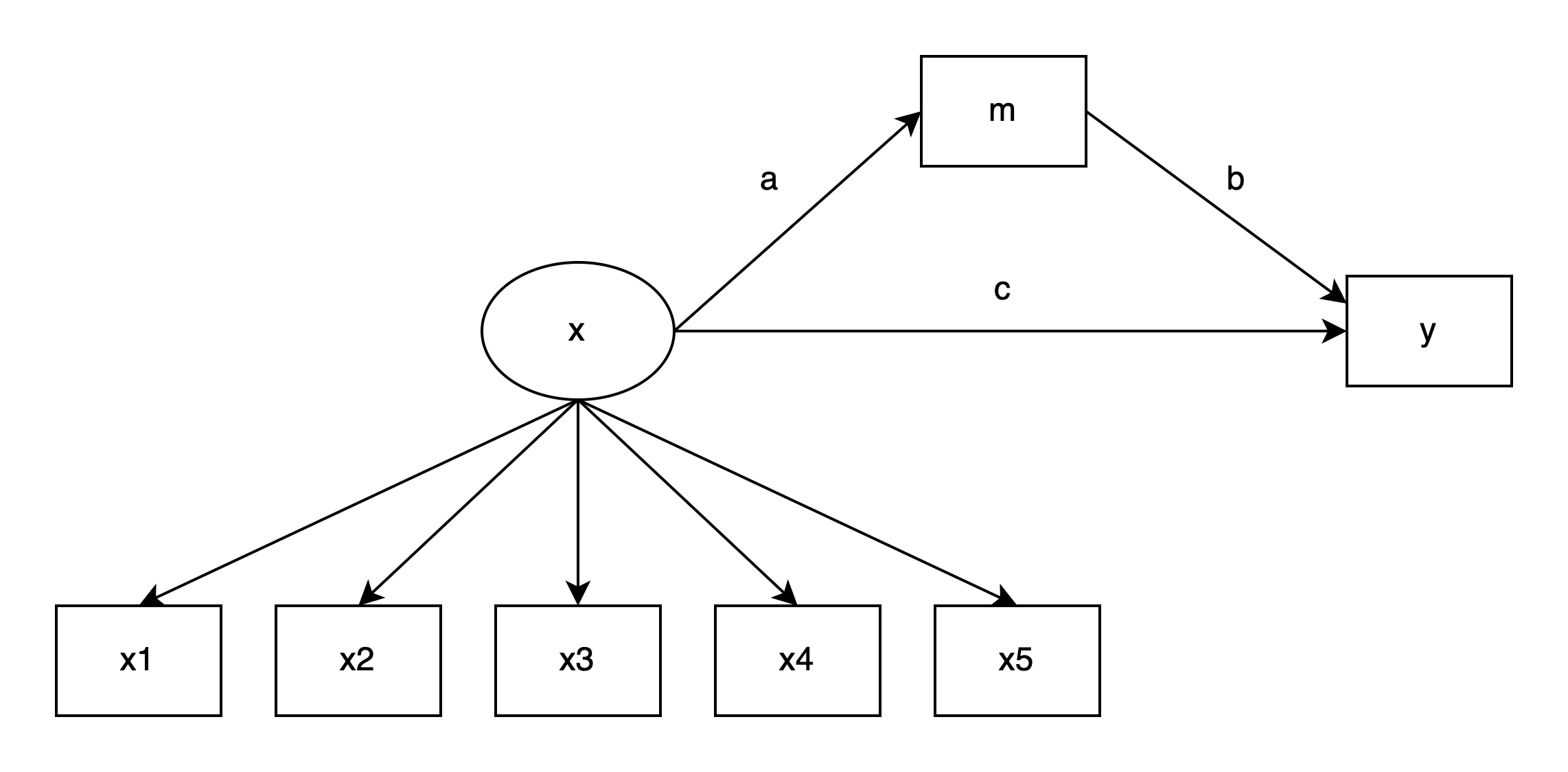
The dataset was simulated to fit a mediation model, where a latent predictor, x, has a direct effect on y and a mediated effect on y through m. This can be represented graphically as follows:
Below is a table of estimates from a mediation model with (1) the complete data and (2) the data after some values in m were made missing, using a listwise deletion procedure. The operators in the “Parameter” column use conventions from the lavaan R package: =~ for latent variable measurement, ~ for regression, ~~ for covariances, and := for calculated quantities of interest.
| Parameter | Estimate | SE | CI | Estimate | SE | CI |
|---|---|---|---|---|---|---|
| x =~ x1 | 1.00 | 0.000 | 1.00 - 1.00 | 1.00 | 0.000 | 1.00 - 1.00 |
| x =~ x2 | 0.83 | 0.099 | 0.63 - 1.02 | 0.90 | 0.120 | 0.66 - 1.13 |
| x =~ x3 | 0.71 | 0.094 | 0.52 - 0.89 | 0.69 | 0.112 | 0.47 - 0.91 |
| x =~ x4 | 0.69 | 0.102 | 0.49 - 0.89 | 0.75 | 0.123 | 0.51 - 0.99 |
| x =~ x5 | 0.62 | 0.105 | 0.42 - 0.83 | 0.65 | 0.126 | 0.41 - 0.90 |
| m ~ x (a) | 1.11 | 0.135 | 0.84 - 1.37 | 1.15 | 0.166 | 0.83 - 1.48 |
| y ~ x (c) | 1.27 | 0.238 | 0.80 - 1.74 | 1.17 | 0.266 | 0.65 - 1.69 |
| y ~ m (b) | 0.75 | 0.140 | 0.48 - 1.03 | 0.82 | 0.151 | 0.52 - 1.11 |
| x1 ~~ x1 | 0.27 | 0.057 | 0.16 - 0.38 | 0.26 | 0.066 | 0.13 - 0.39 |
| x2 ~~ x2 | 0.40 | 0.066 | 0.27 - 0.53 | 0.42 | 0.085 | 0.26 - 0.59 |
| x3 ~~ x3 | 0.41 | 0.064 | 0.28 - 0.53 | 0.45 | 0.083 | 0.29 - 0.61 |
| x4 ~~ x4 | 0.52 | 0.080 | 0.36 - 0.68 | 0.55 | 0.100 | 0.35 - 0.75 |
| x5 ~~ x5 | 0.58 | 0.087 | 0.41 - 0.75 | 0.63 | 0.111 | 0.41 - 0.84 |
| m ~~ m | 0.71 | 0.123 | 0.47 - 0.95 | 0.84 | 0.168 | 0.51 - 1.17 |
| y ~~ y | 0.89 | 0.155 | 0.59 - 1.20 | 0.95 | 0.186 | 0.58 - 1.31 |
| x ~~ x | 0.72 | 0.142 | 0.44 - 1.00 | 0.75 | 0.169 | 0.41 - 1.08 |
| ab := a*b | 0.84 | 0.168 | 0.51 - 1.17 | 0.94 | 0.201 | 0.55 - 1.34 |
| total := c+(a*b) | 2.11 | 0.212 | 1.69 - 2.52 | 2.11 | 0.253 | 1.62 - 2.61 |
| Observations | 100 | 72 |
As expected, under MAR, estimates are biased. Of particular interest is the indirect effect estimate (ab), which differs between the two models.
6.2 Blimp Input
The Blimp script for this analysis is as follows:
DATA: 03_mediation.csv;
LATENT: x;
MODEL:
measurement.model:
x -> x1:x5;
mediation.model:
m ~ x@a;
y ~ m@b x@c;
PARAMETERS:
ab = a * b;
total = ab + c;
SEED: 123;
BURN: 5000;
ITERATIONS: 5000;
Select sections of the script are now discussed.
6.2.1 Named Models
By default, models will appear in the output in alphabetical order by their outcome. To control this, add names before models:
MODEL:
model.name:
outcome ~ predictor;
Then models will appear in the same order in the output as in the script
6.2.2 Additional Parameters
One usage of the PARAMETERS command is to ask Blimp to calculate additional parameters at each iteration. Here, we ask Blimp to calculate the indirect (ab) and total effects from x to y.
In other models we could also calculate things like the difference of two parameters, the predicted value of the outcome under some condition, the variance explained by a single predictor, or the simple slope of a variable in an interaction when the other variable in the interaction is set to some value (e.g., marginal effects, changing reference levels).
6.3 Blimp Output
Running the Blimp script produces this output file:
---------------------------------------------------------------------------
Blimp
3.2.10
Blimp was developed with funding from Institute of
Education Sciences awards R305D150056 and R305D190002.
Craig K. Enders, P.I. Email: cenders@psych.ucla.edu
Brian T. Keller, Co-P.I. Email: btkeller@missouri.edu
Han Du, Co-P.I. Email: hdu@psych.ucla.edu
Roy Levy, Co-P.I. Email: roy.levy@asu.edu
Programming and Blimp Studio by Brian T. Keller
There is no expressed license given.
---------------------------------------------------------------------------
ALGORITHMIC OPTIONS SPECIFIED:
Imputation method: Fully Bayesian model-based
MCMC algorithm: Full conditional Metropolis sampler with
Auto-Derived Conditional Distributions
Between-cluster imputation model: Not applicable, single-level imputation
Prior for random effect variances: Not applicable, single-level imputation
Prior for residual variances: Zero sum of squares, df = -2 (PRIOR2)
Prior for predictor variances: Unit sum of squares, df = 2 (XPRIOR1)
Chain Starting Values: Random starting values
BURN-IN POTENTIAL SCALE REDUCTION (PSR) OUTPUT:
NOTE: Split chain PSR is being used. This splits each chain's
iterations to create twice as many chains.
Comparing iterations across 2 chains Highest PSR Parameter #
126 to 250 1.169 11
251 to 500 1.094 35
376 to 750 1.027 5
501 to 1000 1.011 8
626 to 1250 1.026 5
751 to 1500 1.016 35
876 to 1750 1.026 7
1001 to 2000 1.012 35
1126 to 2250 1.005 49
1251 to 2500 1.022 41
1376 to 2750 1.006 5
1501 to 3000 1.004 26
1626 to 3250 1.006 25
1751 to 3500 1.006 23
1876 to 3750 1.012 5
2001 to 4000 1.004 17
2126 to 4250 1.006 5
2251 to 4500 1.005 36
2376 to 4750 1.004 24
2501 to 5000 1.005 24
DATA INFORMATION:
Sample Size: 100
Missing Data Rates:
x1 = 00.00
x2 = 00.00
x3 = 00.00
x4 = 00.00
x5 = 00.00
m = 28.00
y = 00.00
MODEL INFORMATION:
NUMBER OF PARAMETERS
Outcome Models: 22
Generated Parameters: 2
Predictor Models: 0
FACTORS
Level-1: x
MODELS
measurement.model:
[1] x ~ Intercept@0
[2] x1 ~ Intercept x@1
[3] x2 ~ Intercept x
[4] x3 ~ Intercept x
[5] x4 ~ Intercept x
[6] x5 ~ Intercept x
mediation.model:
[7] m ~ Intercept x@a
[8] y ~ Intercept m@b x@c
GENERATED PARAMETERS
[1] ab = a*b
[2] total = ab+c
WARNING MESSAGES:
No warning messages.
MODEL FIT:
INFORMATION CRITERIA
Marginal Likelihood
DIC2 1850.679
WAIC 1901.957
Conditional Likelihood
DIC2 1850.679
WAIC 1901.957
CORRELATIONS AMONG RESIDUALS:
Summaries based on 5000 iterations using 2 chains.
Correlations Median StdDev 2.5% 97.5% PSR N_Eff
-------------------------------------------------------------------
x, x1 0.032 0.151 -0.265 0.325 1.000 937.633
x, x2 -0.003 0.143 -0.278 0.283 1.001 4658.963
x, x3 -0.003 0.145 -0.281 0.284 1.001 4731.509
x, x4 -0.003 0.147 -0.287 0.279 1.000 5091.989
x, x5 -0.001 0.145 -0.284 0.285 1.001 4952.183
x, m 0.001 0.147 -0.297 0.280 1.000 4671.921
x, y -0.000 0.148 -0.286 0.284 1.000 4475.538
x1, x2 -0.084 0.131 -0.335 0.177 1.000 3234.963
x1, x3 0.070 0.132 -0.203 0.313 1.001 2699.650
x1, x4 0.046 0.127 -0.200 0.285 1.001 3545.896
x1, x5 -0.004 0.127 -0.255 0.245 1.001 3878.584
x1, m 0.029 0.139 -0.247 0.288 1.001 3383.390
x1, y 0.046 0.135 -0.227 0.301 1.001 2793.554
x2, x3 0.037 0.123 -0.205 0.272 1.000 3599.107
x2, x4 -0.010 0.124 -0.248 0.231 1.000 3809.454
x2, x5 0.074 0.119 -0.164 0.298 1.001 3702.143
x2, m 0.085 0.131 -0.183 0.329 1.001 2633.133
x2, y 0.002 0.128 -0.245 0.254 1.000 3772.049
x3, x4 -0.005 0.119 -0.240 0.231 1.000 4278.729
x3, x5 0.129 0.116 -0.106 0.351 1.000 4438.103
x3, m -0.103 0.127 -0.345 0.153 1.002 4102.349
x3, y -0.068 0.125 -0.316 0.179 1.000 3950.181
x4, x5 -0.161 0.116 -0.379 0.073 1.000 4311.600
x4, m 0.047 0.127 -0.206 0.286 1.000 3583.063
x4, y 0.035 0.124 -0.213 0.271 1.000 3888.579
x5, m -0.066 0.124 -0.299 0.179 1.000 4429.844
x5, y 0.019 0.124 -0.225 0.256 1.000 4143.694
m, y 0.001 0.144 -0.279 0.278 1.000 4893.567
-------------------------------------------------------------------
OUTCOME MODEL ESTIMATES:
Summaries based on 5000 iterations using 2 chains.
measurement.model block:
Latent Variable: x
Parameters Median StdDev 2.5% 97.5% PSR N_Eff
-------------------------------------------------------------------
Variances:
Residual Var. 0.701 0.152 0.462 1.050 1.002 553.821
Proportion Variance Explained
by Coefficients 0.000 0.000 0.000 0.000 nan nan
by Residual Variation 1.000 0.000 1.000 1.000 nan nan
-------------------------------------------------------------------
Outcome Variable: x1
Parameters Median StdDev 2.5% 97.5% PSR N_Eff
-------------------------------------------------------------------
Variances:
Residual Var. 0.299 0.064 0.193 0.446 1.006 839.692
Coefficients:
Intercept -0.012 0.101 -0.213 0.178 1.007 406.117
x @1.000 --- --- --- --- ---
Standardized Coefficients:
x 0.834 0.038 0.748 0.897 1.005 422.685
Proportion Variance Explained
by Coefficients 0.695 0.063 0.559 0.804 1.005 421.805
by Residual Variation 0.305 0.063 0.196 0.441 1.005 421.805
-------------------------------------------------------------------
Outcome Variable: x2
Parameters Median StdDev 2.5% 97.5% PSR N_Eff
-------------------------------------------------------------------
Variances:
Residual Var. 0.416 0.074 0.295 0.586 1.000 2470.170
Coefficients:
Intercept -0.015 0.096 -0.199 0.174 1.003 520.860
x 0.854 0.111 0.656 1.089 1.001 619.722
Standardized Coefficients:
x 0.739 0.050 0.622 0.819 1.000 1943.799
Proportion Variance Explained
by Coefficients 0.547 0.072 0.387 0.670 1.000 1892.308
by Residual Variation 0.453 0.072 0.330 0.613 1.000 1892.308
-------------------------------------------------------------------
Outcome Variable: x3
Parameters Median StdDev 2.5% 97.5% PSR N_Eff
-------------------------------------------------------------------
Variances:
Residual Var. 0.424 0.073 0.308 0.596 1.001 2623.750
Coefficients:
Intercept -0.075 0.089 -0.251 0.102 1.005 619.671
x 0.730 0.104 0.544 0.948 1.001 836.071
Standardized Coefficients:
x 0.679 0.058 0.548 0.775 1.000 2274.206
Proportion Variance Explained
by Coefficients 0.461 0.076 0.301 0.601 1.001 2254.319
by Residual Variation 0.539 0.076 0.399 0.699 1.001 2254.319
-------------------------------------------------------------------
Outcome Variable: x4
Parameters Median StdDev 2.5% 97.5% PSR N_Eff
-------------------------------------------------------------------
Variances:
Residual Var. 0.546 0.090 0.404 0.757 1.001 3544.372
Coefficients:
Intercept -0.097 0.095 -0.287 0.084 1.003 685.025
x 0.714 0.113 0.502 0.946 1.000 951.118
Standardized Coefficients:
x 0.624 0.064 0.476 0.728 1.001 3104.569
Proportion Variance Explained
by Coefficients 0.389 0.078 0.227 0.529 1.001 3099.371
by Residual Variation 0.611 0.078 0.471 0.773 1.001 3099.371
-------------------------------------------------------------------
Outcome Variable: x5
Parameters Median StdDev 2.5% 97.5% PSR N_Eff
-------------------------------------------------------------------
Variances:
Residual Var. 0.606 0.096 0.454 0.824 1.000 3765.674
Coefficients:
Intercept -0.008 0.097 -0.196 0.178 1.003 776.068
x 0.646 0.112 0.437 0.875 1.001 1178.967
Standardized Coefficients:
x 0.565 0.069 0.407 0.682 1.001 2913.499
Proportion Variance Explained
by Coefficients 0.319 0.076 0.165 0.465 1.001 2910.447
by Residual Variation 0.681 0.076 0.535 0.835 1.001 2910.447
-------------------------------------------------------------------
mediation.model block:
Outcome Variable: m
Parameters Median StdDev 2.5% 97.5% PSR N_Eff
-------------------------------------------------------------------
Variances:
Residual Var. 0.840 0.173 0.573 1.248 1.001 1698.367
Coefficients:
Intercept 0.024 0.145 -0.258 0.320 1.005 517.072
x 1.179 0.168 0.884 1.536 1.001 634.231
Standardized Coefficients:
x 0.728 0.058 0.596 0.820 1.001 1297.046
Proportion Variance Explained
by Coefficients 0.530 0.082 0.355 0.672 1.001 1284.468
by Residual Variation 0.470 0.082 0.328 0.645 1.001 1284.468
-------------------------------------------------------------------
Outcome Variable: y
Parameters Median StdDev 2.5% 97.5% PSR N_Eff
-------------------------------------------------------------------
Variances:
Residual Var. 0.924 0.177 0.632 1.325 1.000 1731.188
Coefficients:
Intercept -0.220 0.150 -0.510 0.079 1.004 512.879
m 0.737 0.142 0.447 1.005 1.001 1719.590
x 1.304 0.261 0.833 1.844 1.001 1057.096
Standardized Coefficients:
m 0.458 0.085 0.280 0.617 1.000 1706.576
x 0.502 0.086 0.333 0.665 1.001 1654.553
Proportion Variance Explained
by Coefficients 0.799 0.037 0.715 0.861 1.000 1720.223
by Residual Variation 0.201 0.037 0.139 0.285 1.000 1720.223
-------------------------------------------------------------------
GENERATED PARAMETERS:
Summaries based on 5000 iterations using 2 chains.
Parameters Median StdDev 2.5% 97.5% PSR N_Eff
-------------------------------------------------------------------
ab 0.857 0.195 0.513 1.286 1.001 1473.636
total 2.170 0.238 1.749 2.683 1.001 451.043
-------------------------------------------------------------------Select sections of the output are now discussed.
6.3.1 Model Sections
Our script grouped the models into measurement.model and mediation.model, and that is how they appear in the output.
A new section is the “Generated Parameters” at the end, which has the parameters we created in our script. Of note is that the median of the indirect effect ab is very close to that of the frequentist mediation model, indicating that our Blimp model corrected for the bias from the MAR data. However, with the small sample of only 100, our standard errors are quite large, so none of our substantive inferences would have differed.
6.3.2 Model Fit
We typically assess the global fit of mediation and other SEM models through a variety of fit statistics, such as the RMSEA, CFI, and SRMR. Blimp, however, does not include any of these statistics, but adapting such statistics to the Bayesian context is an active area of research.1
Until these statistics are added to Blimp, we have to rely on convergence statistics and nested model comparisons to assess our model fit. Here, our PSR and N_Eff statistics indicate adequate convergence. We have only fit one model here, but we could fit alternative models and use the WAIC values to pick the best model, where lower values indicate better fit.
6.4 Exercise
Fit a mediation model with the dataset exercise_03.csv. (All files are available at this link.) x is the exogenous predictor, and m is the mediator. Create a latent variable from y1, y2, y3, and y4 to serve as the outcome. You have reason to believe m is missing conditional on x. The true indirect effect should be around 0.09.
Asparouhov, T., & Muthén, B. (2021). Advances in Bayesian model fit evaluation for structural equation models. Structural Equation Modeling: A Multidisciplinary Journal, 28(1), 1-14. https://doi.org/10.1080/10705511.2020.1764360↩︎