| Variable | Estimate | SE | t | p | 95% CI Lower | 95% CI Upper |
|---|---|---|---|---|---|---|
| x | 1.02 | 0.45 | 2.27 | 0.01 | 0.14 | 1.90 |
2 Bayesian Basics
In this chapter, we will first review frequentist inference, discuss how Bayesian inference offers an alternative, and then go through the very basics of Bayesian statistics. To learn more, see the Resources section.
2.1 Direction of Inferences
If you have not heard of Bayesian statistics before, chances are that you have been doing frequentist statistics. Frequentist statistics is concerned with long-run probabilities and has particular ways of talking about statistical inference.
Quiz time!
Imagine we ran a regression predicting y from x, and this was one of the lines in our regression output:
What does the p-value of 0.01 mean?
A. There is a 1% chance we would observe this test statistic by chance.
B. There is a 1% chance the true relationship between x and y in the population is zero.
C. There is a 1% chance of observing a test statistic greater than or equal to this one if the true relationship between x and y is zero.
What does the 95% confidence interval of [0.14, 1.90] mean?
A. There is a 95% chance the true relationship between x and y is between 0.14 and 1.90.
B. If we resample from the population and rerun the model many times, 95% of the confidence intervals will include the true population value.
C. If we resample from the population and rerun the model many times, 95% of the estimates will fall between 0.14 and 1.90.
Click here to see the answers
C
B
Explanation of 1: Our p-value tells us the probability of observing our data while assuming the null hypothesis is true. We evaluate the probability of our data, not the probability of our null hypothesis. We make inferences about our sample, not the population.
Explanation of 2: Population parameters are unknown, fixed quantities. We cannot speak of the probability of them being in some range; they are either inside our confidence interval, or they are outside of it. We can only argue that, assuming our model is correct, that the population parameter will be inside 95% of the confidence intervals constructed from repeated sampling. (On that note, it is striking how frequentist statistical inference is built upon repeated sampling and replication, but there is a severe lack of replication studies in the literature of many fields.)
However, we usually do research because we want to estimate population parameters. We ask, “How much more effective is Drug A than Drug B?” rather than, “What is the probability of observing this difference in effectiveness between Drug A and Drug B if there is actually no difference?” We want to know the probability of a hypothesis being true given our data, not the probability of our data assuming some hypothesis is true.
A small p-value is often thought to justify a statement of the sort “having looked at these data, I believe that hypothesis H0 is quite implausible.” Of course, and as I detail below, this is not what a p-value is: the p-value is a statement about the plausibility of the data (and other, more extreme, but hypothetical unobserved data sets) conditional on a null hypothesis. Adopting an explicitly Bayesian approach would resolve a recurring source of confusion for these researchers, letting them say what they mean and mean what they say.1
To reverse the direction of our inferences, to go from sample to population instead of population to sample, we can use Bayes’ theorem.
2.2 Bayes’ Theorem
Bayes’ theorem can be stated as
\[ P(\theta|x) = \frac{P(x|\theta)P(\theta)}{P(x)} \]
where
- \(\theta\) is some parameter
- \(x\) is our data
- \(P(\theta|x)\) is the posterior probability of some parameter given our data
- \(P(x|\theta)\) is the likelihood of our data given some parameter
- \(P(\theta)\) is the prior probability of some parameter
- \(P(x)\) is the probability of our data
The denominator (\(P(x)\)) only serves to normalize the probability, so removing that yields
\[ P(\theta|x) \propto P(x|\theta)P(\theta) \]
where \(\propto\) means “propotional to.” In words, this equation means that “the posterior is proportional to the prior times the likelihood.”2
In other words, instead of talking about the likelihood of our data given some parameter (\(P(x|\theta)\)) as in frequentist inference, we can talk about the probability of some parameter given our data (\(P(\theta|x)\)) because we introduced the prior of that parameter (\(P(\theta)\)).
2.3 Priors
A prior is a probability distribution that captures what we believe about our parameters before (prior to) collecting our data. Every parameter in a Bayesian statistical model has a prior: the intercept, coefficient estimates, variances, covariances, R2, random slopes, and so on. Priors provide a way to include information from the literature and expert opinion. We might believe a parameter is in some specific range with certain probabilities of certain values (an “informative prior”), or we may have a vague or no idea how it is distributed (an “uninformative prior”).
Blimp automatically selects suitable uninformative priors based on the variable types and model form, but it does allow manual specification of priors. For more fine-grained control, use a package like RStan.
2.4 Chains and Distributions
Notice how the left side of Bayes’ theorem gives us a posterior probability distribution, rather than a point estimate. How is that distribution mapped out?
Bayesian estimation uses an iterative process. First, random starting values for parameters are chosen. Second, the likelihood probability is updated. Third, parameter values are estimated. These parameter estimates allow us to then pick new plausible values, which updates the likelihood, which yields new parameter estimates, which allows us to pick new values, and so on. This process is repeated hundreds or thousands (or more) of times in a process called Markov chain Monte Carlo, or MCMC for short. MCMC is a method for sampling from a probability distribution (recall that Bayes’ theorem is all about probability distributions). See this blog post for an intuitive explanation of how MCMC sampling works.
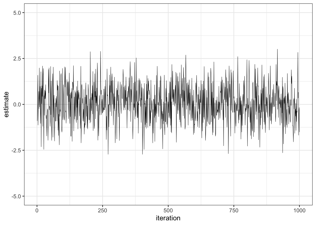
We typically visualize MCMC with trace plots. In this plot, we sampled from a normal distribution and plotted the values against the iteration number:
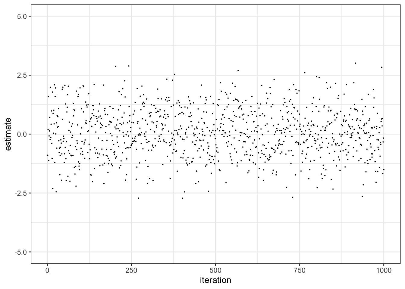
A trace plot is just points that have been connected. Removing the lines gives us this plot:
Now, let’s take that plot and rotate is 90 degrees. Imagine that each point is a grain of sand, and we allow them to fall with gravity. The result would be a pile of sand with some shape: a distribution.

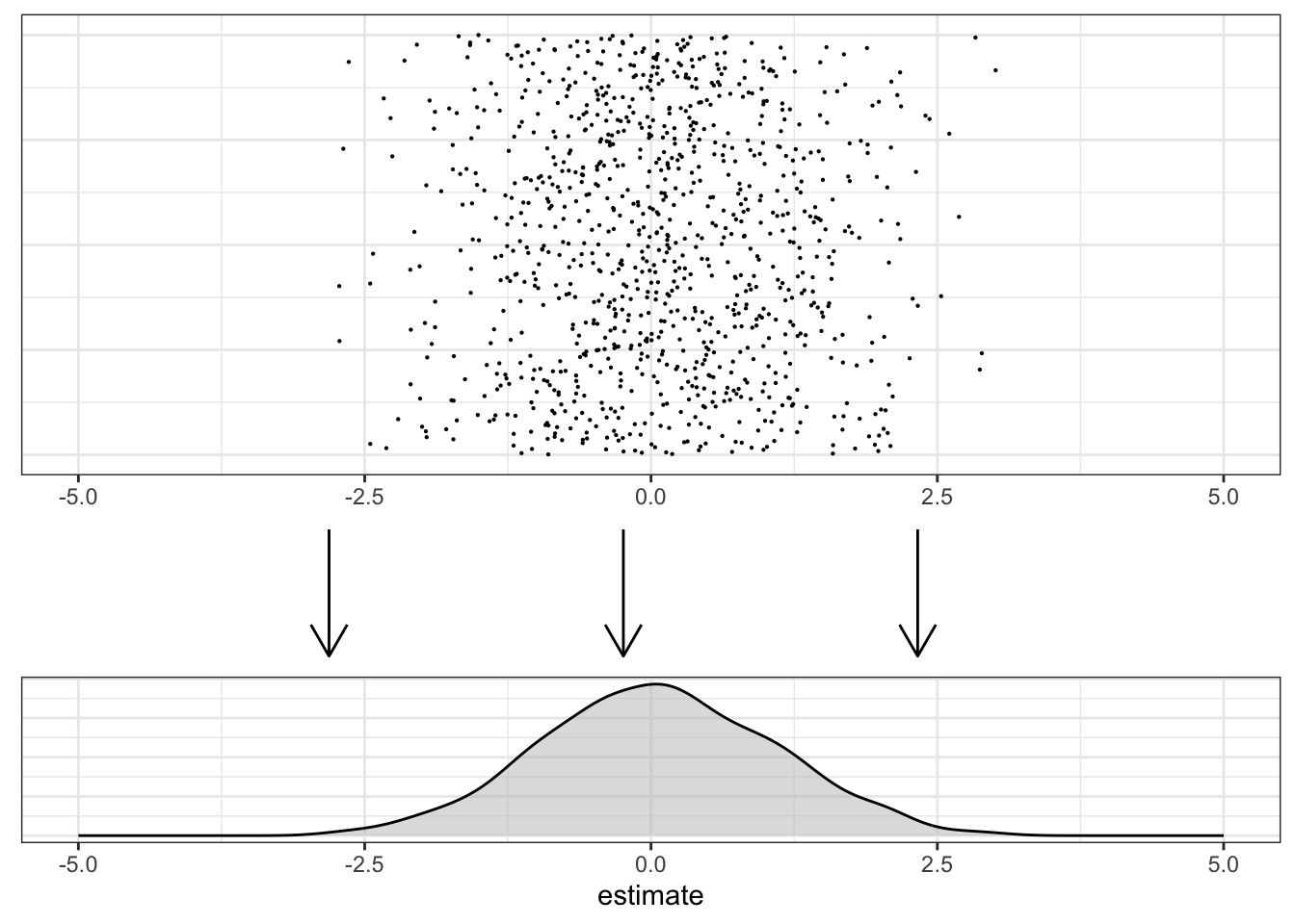
We usually summarize our posterior distribution with two types of statistics:
- Some measure of central tendency (e.g., median, mean)
- Some measure of variability (e.g., standard deviation, 95% quantile interval)
2.5 Bayesian Inference
Bayesian inference conceives of parameters as unknown, random quantities, and it does not depend on long-run frequencies.
We can then do what we wished we could do in frequentist inference. In a Bayesian framework, we can make inferences about parameters based on our posterior distribution. Bayesian inference allows researchers to “say what they mean and mean what they say.”3
We summarize our posterior with a statement of probability about a parameter, and we use a 95% credible interval. A credible interval is similar in calculation to a confidence interval, but we intepret it very differently. If our 95% credible interval for some parameter is [0.14, 1.90], we can say there is a 95% probability the true population value is somewhere in that range.
If we flip a (fair) coin and ask a frequentist and a Bayesian about the probability that it is heads without showing them the result, we would get fundamentally different interpretations of probability. The frequentist would say, “It is either heads or tails. If we flip the coin many, many times, we would expect that 50% of the flips would be heads, but I cannot say anything about this particular flip.” The Bayesian would say, “There is a 50% probability the coin is heads.”
2.6 Bayesian Missing Data Analysis
Blimp allows us to leverage Bayesian statistical modeling for missing data analysis. It will be helpful to compare Blimp’s approach with multiple imputation.
Both approaches seek to correct the bias that can arise from missing data, use MCMC chains to iteratively estimate multiple plausible values for missing values, and recognize our uncertainty regarding the true value of those missing values.
Both use random starting values, estimate models, impute plausible missing values, re-estimate models, re-impute, and so on. The difference is that multiple imputation only keeps the sets of imputed values (perhaps 20 or 50 or 100) for use in frequentist models. Blimp, on the other hand, saves the estimates from the model in each iteration, and uses those to construct the posterior probability. (Blimp also allows you to export imputed datasets for use in frequentist analyses in other programs.)
In the next chapters, we will become familiar with the Blimp interface and its scripting language.