2 Functions

First, load the tidyverse.

library(tidyverse)

2.1 Turning Procedures into Functions

A procedure is one or more lines of code we run to do things like calculate summary statistics, transform variables, and read and write files. Our existing code serves as raw material we can transform into functions, which makes it portable and allows us to reuse it within and across scripts with minimal repetition.

Tip

If you want to reuse a procedure more than two or three times, turn it into a function.

2.1.1 Example: Calculating the Standard Error

In the code below, we calculate the standard error (\(\frac{SD_x}{\sqrt{n}}\) ) of several columns in mtcars, which involves repeating the same procedure for several different R objects.

sd(mtcars$mpg) / sqrt(length(mtcars$mpg))

[1] 1.065424

sd(mtcars$wt) / sqrt(length(mtcars$wt))

[1] 0.1729685

sd(mtcars$hp) / sqrt(length(mtcars$hp))

[1] 12.12032

The functions are the same, but the objects vary.

Two things change in each line: the object inside of sd() and the object inside of sqrt(length()), which are the same object within each line. Fill them in with a placeholder, x:

sd(x) / sqrt(length(x))

Now, to turn this procedure into a function, we need (1) a name and (2) the number of arguments, with suitable names.

For the name of the function, se is concise and meaningful, but we should first check if it is the name of another existing function in a library we have loaded at the moment:

?se

No documentation for 'se' in specified packages and libraries:
you could try '??se'

That means it is not already used, so we will not have any naming conflicts if we were to use this name.

For the arguments, we only have one argument, which we can keep calling x. If we had multiple arguments or planned on using a function more often, we should give the arguments more informative names. For now, x is fine.

The structure of our function-making syntax is as follows:

function_name <- function(argument) {
  procedure
}

If we replace function_name, argument, and procedure with their values, we get this code:

se <- function(x) {
  sd(x) / sqrt(length(x))
}

Running that line will add se() to our global environment under the Functions header, so that is available for our use. Now let’s use it!

se(mtcars$mpg)

[1] 1.065424

se(mtcars$wt)

[1] 0.1729685

se(mtcars$hp)

[1] 12.12032

2.1.2 Example: Counting Missing Values

As another example, let’s get the number of missing values in a vector:

sum(is.na(airquality$Ozone))

[1] 37

sum(is.na(airquality$Solar.R))

[1] 7

What changes in each line? Replace that with x:

sum(is.na(x))

Name the function nmiss and fill in the function template:

nmiss <- function(x) {
  sum(is.na(x))
}

Now use it:

nmiss(airquality$Ozone)

[1] 37

nmiss(airquality$Solar.R)

[1] 7

2.2 Exercises: Basic Functions

The code below returns the proportion of rows in a dataframe that do not have any missing data. Create a function called prop_observed() that does the same.

nrow(na.omit(txhousing)) / nrow(txhousing)

[1] 0.828412

nrow(na.omit(storms)) / nrow(storms)

[1] 0.1110713

prop_observed(txhousing)

[1] 0.828412

prop_observed(storms)

[1] 0.1110713

The following line returns how many years have passed since some date given in year-month-day format. In this example, we use July 20, 1969, the Apollo 11 moon landing.
```
time_length(interval(ymd(19690720), Sys.Date()), unit = "years")
```
```
[1] 55.06575
```
Create a function called years_since() that does the same, and use it to find how many years have passed since some significant dates for you, like a birthday, wedding, or starting your graduate school. (Note the ymd() function works with dates in various year-month-day formats, everything from 19690720 to 1969-07-20 to "1969 July 20". For working with dates, see our chapter on date vectors.)
```
years_since(19690720)
```
```
[1] 55.06575
```

The code below prints a greeting.

cat(paste0("Good morning, ", "Jason", ".\nToday is ", format(Sys.Date(), "%B %d, %Y"), ".\n"))

Good morning, Jason.
Today is August 13, 2024.

Create a function called morning() that takes the user’s name.

morning("World")

Good morning, World.
Today is August 13, 2024.

2.3 Environments

Most of our work in R involves working with objects in the global environment. This is the one we see in the top-right Environment pane of RStudio, and the objects there are available to everything in our current session. Other environments exist, and functions actually execute in their own environment.

The technical details of environments are discussed elsewhere¹, so here we will focus on the implications for our function writing. Keep these three things in mind:

Objects created within functions with <- are not stored in the global environment.
Each time a function is run, it runs in a new environment.
A function searches its own environment before it searches the global environment.

We will discuss each of these in turn.

2.3.1 Objects created within functions

Let’s create a somewhat useful function that reports the empirical standard deviation from a random sample drawn from a normal distribution of size n. The expected standard deviation, per the default of rnorm(), is 1. The error tends to get smaller as the sample size increases.

empirical_sd <- function(n) {
  sample_data <- rnorm(n)
  sd(sample_data)
}

empirical_sd(10)

[1] 0.780586

empirical_sd(10000)

[1] 1.012406

empirical_sd(1000000)

[1] 1.000062

Take a look at the procedure inside the function. We make an object, sample_data, and then calculate and print the standard deviation.

Does sample_data exist in our global environment?

"sample_data" %in% ls()

[1] FALSE

No. It only exists within the function’s environment. Functions do not return intermediary assigned objects; instead, they return the result of the last expression.

2.3.2 Functions run in new environments

Not only do functions run in their own environments, they run in a new environment each time.

The function add_one() has no arguments, and it simply adds one to the object i. We initialize it with a value of 1. After the first call of add_one(), i is 2. We may expect that i increases each time, but it does not.

add_one <- function() {
  i <- i + 1
  i
}

i <- 1

add_one()

[1] 2

add_one()

[1] 2

add_one()

[1] 2

The reason for this is that our global environment has i with a value of 1. The first call of add_one() creates an environment, gets i from the global environment, and adds 1 to it, so that i is now 2. The next call of add_one() does not see the environment from the previous call of the function, so it gets i with a value of 1 from the global environment, adds 1 to make 2, and so on.

The function will search its own environment before searching the global environment. The upside of this is that we do not need to worry about conflicts between function argument names and our global environment.

2.3.3 Environment Search Order

To illustrate the search order of functions, let’s modify the add_one() code from above to include the line i <- 10. The output is 11 because add_one() finds the i with a value of 10 in its own environment before finding the i with a value of 1 in the global environment.

add_one <- function() {
  i <- 10
  i <- i + 1
  i
}

i <- 1

add_one()

[1] 11

The upside of this is that we do not need to worry about conflicts between the names of objects in our function, and the names of objects in our global environment. That is, while in general we need to thoughtfully name our objects, we are also free inside our functions to call every vector x or y and every dataframe dat or df.

2.4 Multiple Returns

Given that assigning objects within functions does not assign objects in our global environment, and our last returned object is returned, how can we return multiple objects?

Let’s add to nmiss() to also give the total number of values and the proportion of missing values:

miss_stats <- function(x) {
  length(x)
  sum(is.na(x))
  mean(is.na(x))
}

miss_stats(airquality$Ozone)

[1] 0.2418301

Only the last value is returned, mean(is.na(x)).

A solution is to make a (named) list that contains all the objects we want returned. Lists are excellent containers when you want to return a variety of objects since they can contain objects of different types and structures.

miss_stats <- function(x) {
  list(n = length(x),
       miss_count = sum(is.na(x)),
       miss_prop = mean(is.na(x)))
}

miss_stats(airquality$Ozone)

$n
[1] 153

$miss_count
[1] 37

$miss_prop
[1] 0.2418301

2.5 Arguments and Defaults

If we use more informative argument names, our functions become easier to use and later understand.

The code below takes proportions (0-1) and turns them into percentages (0-100%) with a differing numbers of decimal places.

x <- seq(0, 1, .1243)
y <- seq(0, 1, .2345)

[1] 0.0000 0.1243 0.2486 0.3729 0.4972 0.6215 0.7458 0.8701 0.9944

[1] 0.0000 0.2345 0.4690 0.7035 0.9380

trimws(paste0(format(round(x * 100, 2), nsmall = 2), "%"))

[1] "0.00%"  "12.43%" "24.86%" "37.29%" "49.72%" "62.15%" "74.58%" "87.01%"
[9] "99.44%"

trimws(paste0(format(round(y * 100, 1), nsmall = 1), "%"))

[1] "0.0%"  "23.4%" "46.9%" "70.3%" "93.8%"

In these, we have two pieces that change: the vector (x, y) and the number of decimal places (1, 2), which occures twice. We can use x for the vector argument name and n_decimal for the number of decimal places argument name.

trimws(paste0(format(round(x * 100, n_decimal), nsmall = n_decimal), "%"))

The first line of our code to create that function will look like this:

prop_to_perc <- function(x, n_decimal) {

We may find that we often want to round to two decimal places, so we should set that as an argument default. Defaults are set with the pattern argument = value:

prop_to_perc <- function(x, n_decimal = 2) {

Now, reformat the code inside the function with pipes to make it more readable.

prop_to_perc <- function(x, n_decimal = 2) {
  round(x * 100, n_decimal) |> 
    format(nsmall = n_decimal) |> 
    paste0("%") |> 
    trimws()
}

Now use the function on x and y. For x, we are fine with the default of 2 decimal places, so we do not need to specify anything.

prop_to_perc(x)

[1] "0.00%"  "12.43%" "24.86%" "37.29%" "49.72%" "62.15%" "74.58%" "87.01%"
[9] "99.44%"

And for y, we want just 1 decimal place, so we need to specify that:

prop_to_perc(y, n_decimal = 1)

[1] "0.0%"  "23.4%" "46.9%" "70.3%" "93.8%"

Following our earlier discussion of environments, note how each function call finds the x in its own environment instead of the x in the global environment.

2.6 Conditionals

Sometimes we may want a single function that does different things with different types of input.

For example, take the function plot(). If we give it a numeric vector, it gives us a scatterplot of values by index:

plot(chickwts$weight)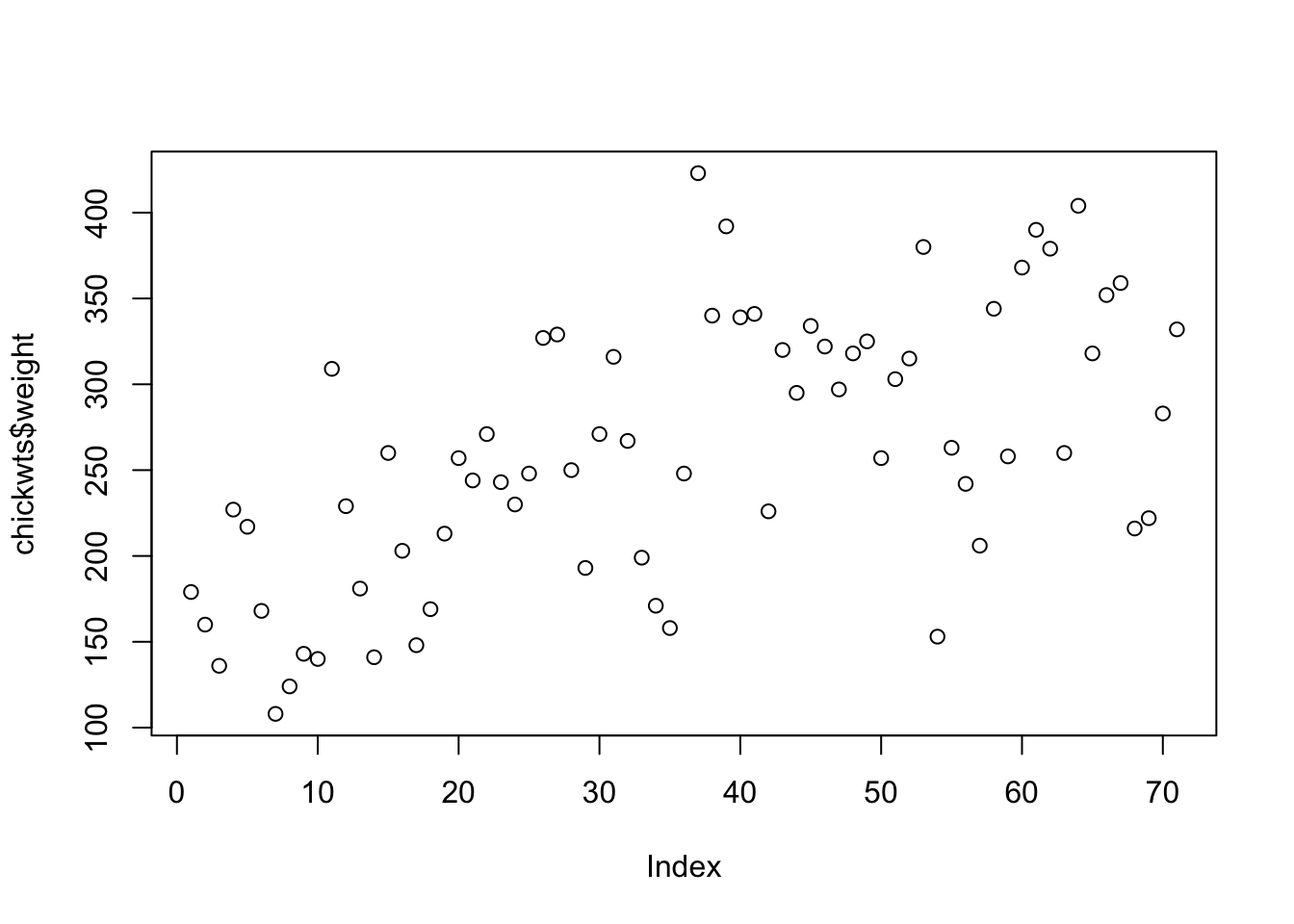

And if we give it a factor, it returns a bar chart:

plot(chickwts$feed)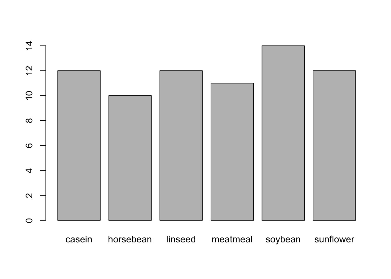

But it fails if we give it a character vector:

plot(as.character(chickwts$feed))

Warning in xy.coords(x, y, xlabel, ylabel, log): NAs introduced by coercion

Warning in min(x): no non-missing arguments to min; returning Inf

Warning in max(x): no non-missing arguments to max; returning -Inf

Error in plot.window(...): need finite 'ylim' values

And if we give it a logical vector, it returns a plot where TRUE and FALSE have been coerced to 1 and 0, respectively:

plot(chickwts$weight > 250)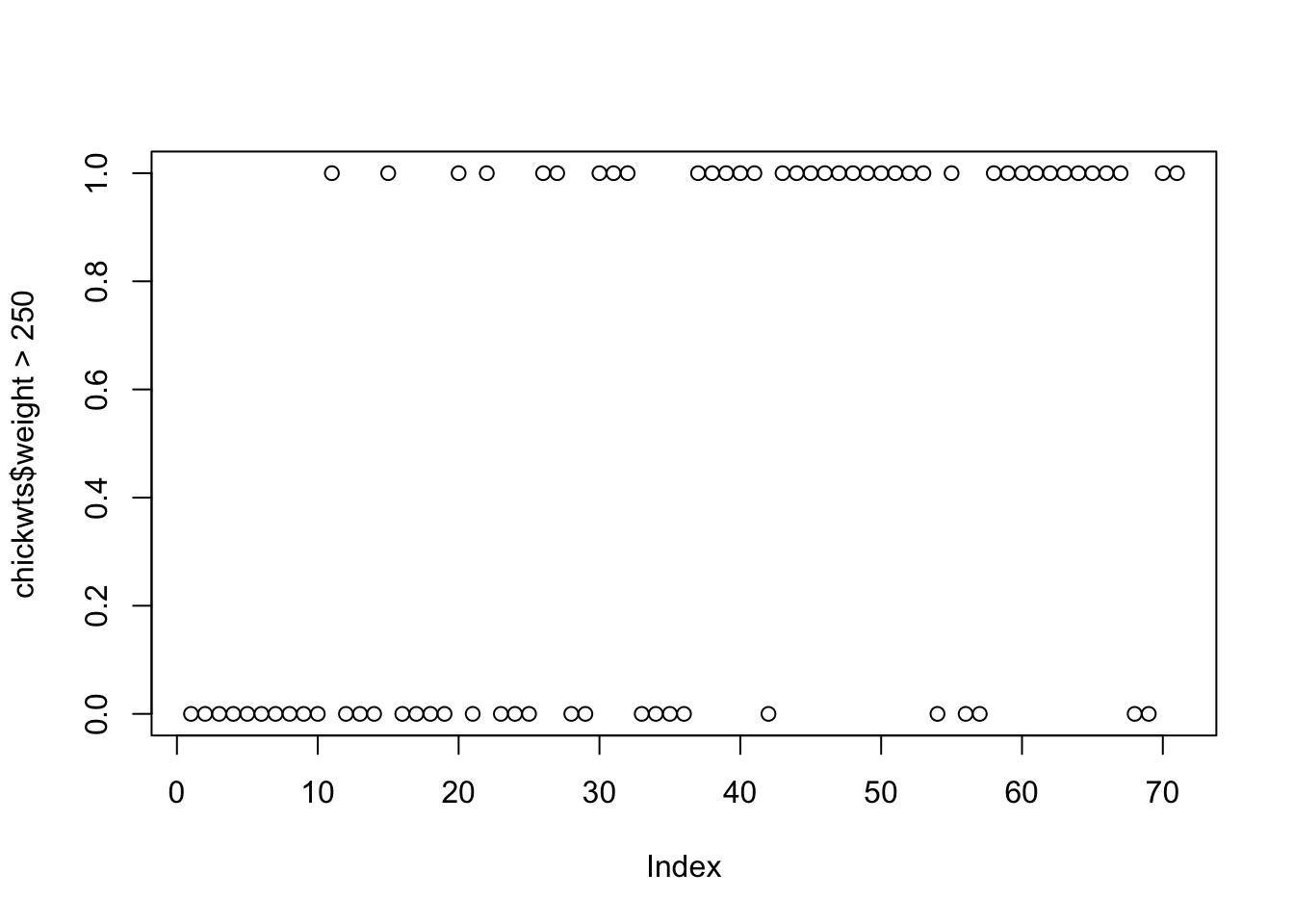

Let’s make a function that plots vectors of different types. It can return the default plots for numeric and factor vectors, but for character and logical vectors, it should coerce them to factor vectors first.

We should also limit the function to only work with vectors so that we do not get unexpected results with other data structures and objects. To do this, we can use stopifnot() with a condition: check if it is a vector or a factor (which technically is not a vector…):

stopifnot(is.vector(x) | is.factor(x))

After that, we need branching logic. If it is a character or logical vector, make it a factor and then plot it. Otherwise, plot it as-is:

if (is.character(x) | is.logical(x)) {
  plot(as.factor(x))
} else {
  plot(x)
}

Put this all together inside a function which we can call plot_vec():

plot_vec <- function(x) {
  stopifnot(is.vector(x) | is.factor(x))
  
  if (is.character(x) | is.logical(x)) {
    plot(as.factor(x))
  } else {
    plot(x)
  }
}

And now test it with a few inputs:

plot_vec(chickwts$weight) # numeric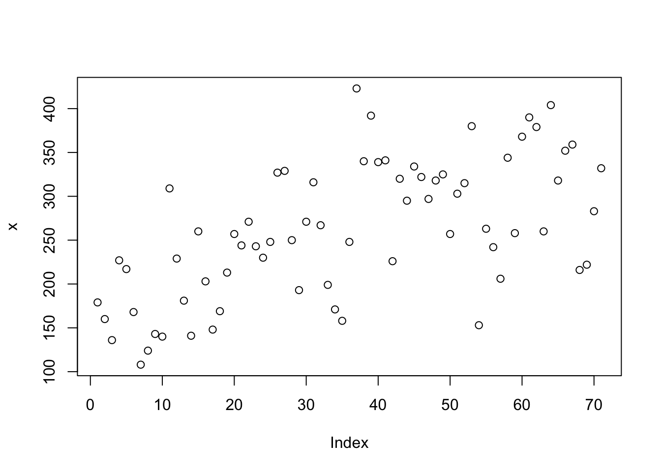

plot_vec(chickwts$feed) # factor

plot_vec(as.character(chickwts$feed)) # character

plot_vec(chickwts$weight > 250) # logical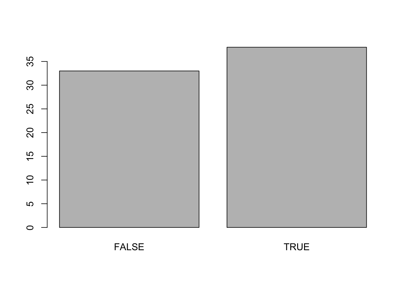

Now give it another data structure to see how it reacts:

plot_vec(mtcars)

Error in plot_vec(mtcars): is.vector(x) | is.factor(x) is not TRUE

It is working as expected, but we could improve that error message.

We can change from using stopifnot() to using an if statement with our condition along with stop(), which can contain a more helpful error message. It can tell the user the structure of the provided object and instruct them to instead supply a vector.

plot_vec <- function(x) {
  if (!(is.vector(x) | is.factor(x))) {
    stop(paste("x is a", class(x)[[1]], "but it should be a vector"))
  }
  
  if (is.character(x) | is.logical(x)) {
    plot(as.factor(x))
  } else {
    plot(x)
  }
}

Now try it out:

plot_vec(mtcars)

Error in plot_vec(mtcars): x is a data.frame but it should be a vector

2.7 Tidyverse Functions

tidyverse functions usually make code easier to read and write because we do not need to repeat the dataframe name each time²:

df$var3 <- 
  df$var1 + df$var2

df <- 
  df |> 
  mutate(var3 = var1 + var2)

In the context of functions, however, using tidyverse functions requires extra work since we need to explicitly tell them to look within the dataframe to find the variables.

To illustrate the problem, here we make a function called wrong() that tries to get the mean of a given variable, but it fails to find mpg since it does not know to look inside mtcars. Adding quotes around the variable name does not solve the issue either.

wrong <- function(df, var) {
  df |> summarize(mean = mean(var))
}
wrong(mtcars, mpg)

Warning: There was 1 warning in `summarize()`.
ℹ In argument: `mean = mean(var)`.
Caused by warning in `mean.default()`:
! argument is not numeric or logical: returning NA

  mean
1   NA

wrong(mtcars, "mpg")

Warning: There was 1 warning in `summarize()`.
ℹ In argument: `mean = mean(var)`.
Caused by warning in `mean.default()`:
! argument is not numeric or logical: returning NA

  mean
1   NA

This issue can be solved in one of two ways within our function:

Embrace the variable name with double curly braces: {{ var }}. See right1() below.
Use the .data pronoun with a character vector: .data[[var]]. See right2() below.

right1 <- function(df, var) {
  df |> summarize(mean = mean({{ var }}))
}
right1(mtcars, mpg)

      mean
1 20.09062

right2 <- function(df, var) {
  df |> summarize(mean = mean(.data[[var]]))
}
right2(mtcars, "mpg")

      mean
1 20.09062

When would we use one over the other?

{{ var }} is useful when we specify variable names in function arguments

.data[[var]] is useful when we have a character vector returned by something else, like user input from a Shiny app or output from some other code like

myVar <- colnames(mtcars)[[1]]
myVar

[1] "mpg"

2.7.1 Embracing

We often need to calculate custom summary statistics for variables in our data. The code below takes a dataframe and variable as arguments, so we need to embrace the variable name in the function syntax:

mySummary5 <- function(df, var) {
  df |> 
    summarize(n = n(), 
              mean = mean({{ var }}, na.rm = T), 
              median = median({{ var }}, na.rm = T), 
              sd = sd({{ var }}, na.rm = T), 
              se = sd({{ var }}, na.rm = T) / sqrt(n()))
}

mySummary5(airquality, Temp)

    n     mean median      sd        se
1 153 77.88235     79 9.46527 0.7652217

mySummary5(airquality, Ozone)

    n     mean median       sd       se
1 153 42.12931   31.5 32.98788 2.666912

(Note that we could have used .data[[var]] within the function and then specified “Temp” and “Ozone” in the function calls.)

2.7.2 The .data Pronoun

In this example, let’s fit a regression model and then produce plots to assess the linearity assumption. Because we want to specify the variable names as character vectors, we need to specify .data[[var]] within the function.

mod <- lm(mpg ~ wt + disp + drat, mtcars)

linearity_plot <- function(df, mod, var) {
  df <-
    df |> 
    mutate(res = residuals(mod),
           yhat = fitted(mod))
  
  ggplot(df, aes(.data[[var]], res)) +
    geom_point() +
    geom_hline(yintercept = 0, color = "red") +
    geom_smooth()
}

Now use the function to plot the fitted values and each predictor (just wt here, but we should check all of them):

linearity_plot(mtcars, mod, "yhat")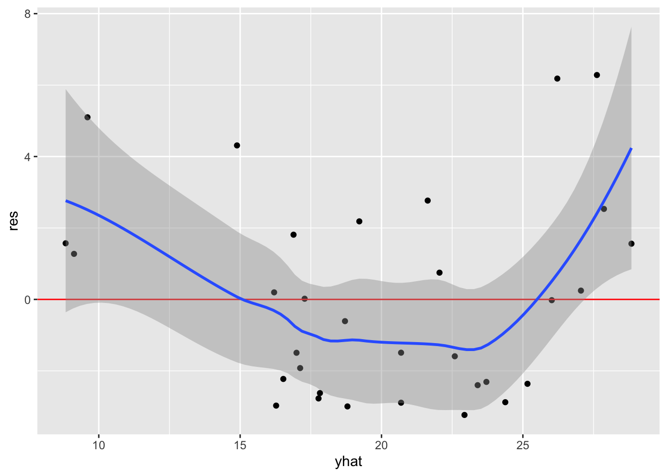

linearity_plot(mtcars, mod, "wt")

(Note we could have used embracing ({{ var }}) in the function and then referred to the vars as yhat and wt in the function calls.)

To show where we will go in the next chapter on Iteration, we can first programmatically extract the names of our predictors and then iteratively plot them with map():

predictors <- colnames(model.frame(mod))[-1]
predictors

[1] "wt"   "disp" "drat"

map(predictors, \(x) linearity_plot(mtcars, mod, x))

[[1]]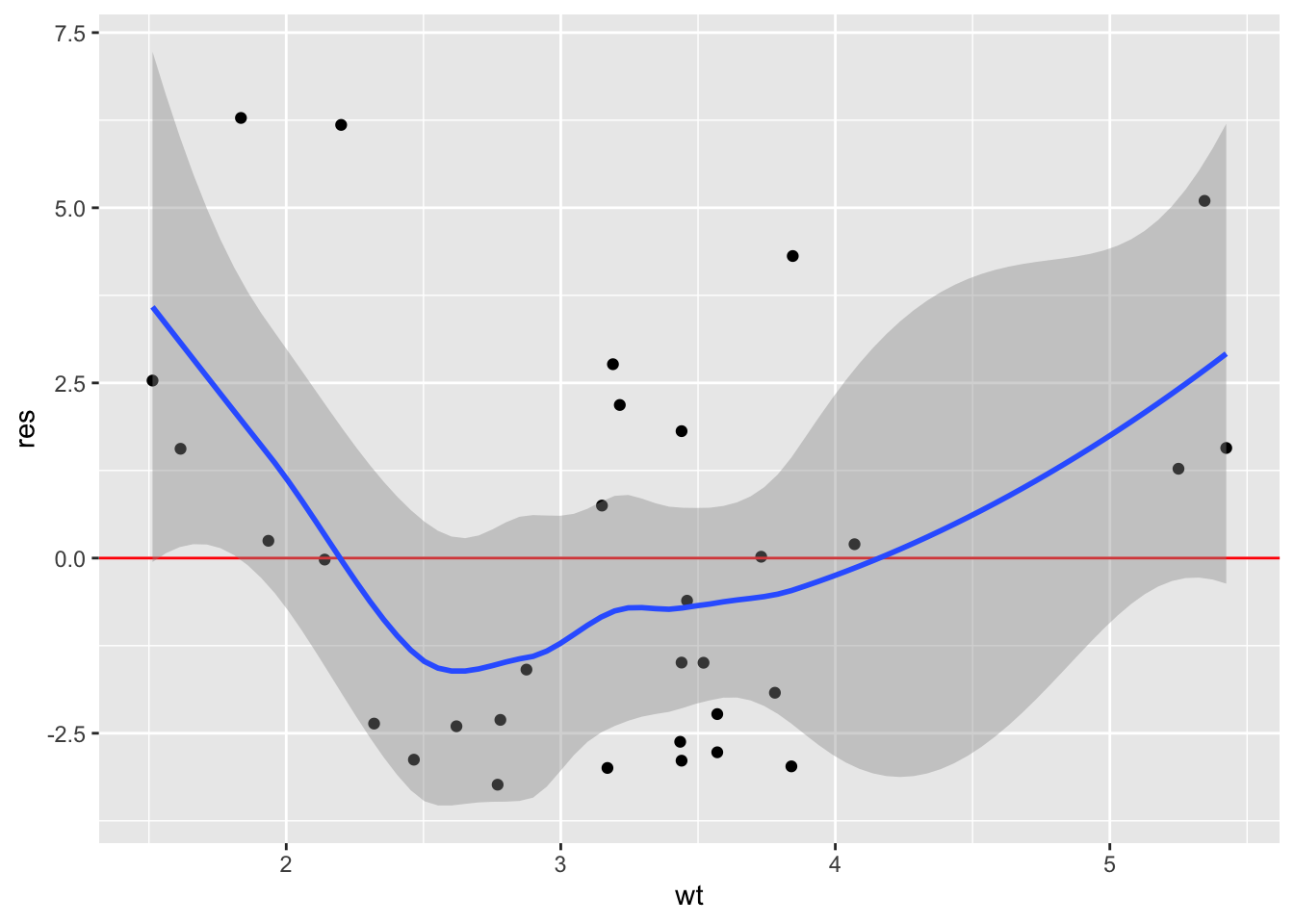


[[2]]


[[3]]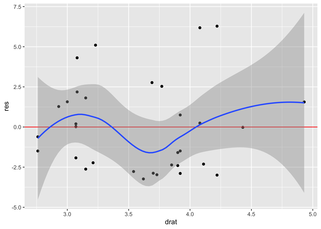

2.8 Reusing Functions Across Scripts

We may find that some functions we write are actually quite useful, and we want to use them across projects. We know we should not copy and paste code again and again within a script, but what about between scripts? How can we make a function available to multiple projects?

We have two options: creating a script with functions, and writing a package. Package writing is outside the scope of this resource. Packages can be used locally without publishing them, but it would be quite an addition to your resume to publish packages to GitHub or even CRAN. See R Packages to learn more.

For now, let’s just put our functions inside a script somewhere on our computer. We then need to “source” that script. Just add a line to the beginning of your script where you load other libraries:

library(tidyverse)
source("path/to/file/myFunctions.R")

source() will run a script. Any functions or objects created in that script will be added to the global environment, and then you can use them in your current project.

2.9 Exercises: Complex Functions

Revisit the time difference calculator from the previous exercises. Modify the function so that the units (years, months, days, etc.) can be specified.
```
time_since(19690720, "days")
```
```
[1] 20113
```
Sometimes, missing is coded with more than one missing code. Write a function that uses ifelse() and returns a vector after replacing specified values with NA. For example, if 8 and 9 are missing codes, this vector:
```
set.seed(2)
x <- sample(c(1:3, 8, 9), 10, replace = T)
x
```
```
 [1] 9 1 9 1 8 9 1 2 3 1
```
should be returned as:
```
to_na(x, 8:9)
```
```
 [1] NA  1 NA  1 NA NA  1  2  3  1
```
Fix this function. The problem is that the output does not vary.

get_sample() should return a sample of size n. Fix it so that get_sample(3) returns 3 values. Refer to ?sample.
```
get_sample <- function(n) {
  sample(1:5, replace = T)
}

get_sample(3)
```
```
[1] 3 2 3 1 1
```

Fix this function. The problem is that there is no output.

fit_mod() should return a fitted model object, but nothing is returned.

fit_mod <- function(df, outcome, predictors) {
  form <- 
    as.formula(
      paste(outcome, 
            "~",
            paste(predictors, collapse = "+")
      )
    )
  mod <- lm(form, data = df)
}

fit_mod(df = mtcars, 
        outcome = "mpg",
        predictors = c("wt", "disp", "wt*disp"))

Fix this function. The problem is that the scatterplot only shows one point.

scatter() should produce a scatterplot of a given x and y from dataframe df.
```
scatter <- function(df, x, y) {
  ggplot(df, aes(x, y)) +
    geom_point()
}

scatter(mtcars, "wt", "mpg")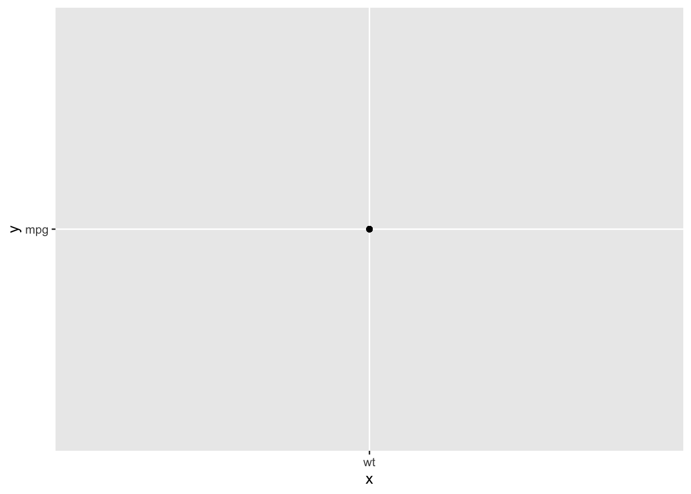
```

To learn more about environments in R, see the “Environments” chapters of Advanced R and Hands-On Programming with R.↩︎
Due to data masking and tidy evaluation.↩︎