8 No Outlier Effects
What this assumption means: Our statistical model accurately represents the relationships in the data.
Why it matters: Outliers, which are observations whose values greatly differ from those of other observations, sometimes have disproportionately large influence on the predicted values and/or model parameter estimates.
How to diagnose violations: Large values of DFFITS and/or DFBETAS.
How to address it: Examine influential observations and investigate why they are outliers. Add predictors to the model.
8.1 Example Model
If you have not already done so, download the example dataset, read about its variables, and import the dataset into R.
Then, use the code below to fit this page’s example model.
acs <- readRDS("acs2019sample.rds")
mod <- lm(income ~ age * sex + hours_worked + weeks_worked, acs, na.action = na.exclude)
8.2 Statistical Tests
Outliers can be classified into three types:
- Extreme values
- Leverage
- Influence, which can be divided into two types:
- Influence on predicted values
- Influence on parameter estimates
8.2.1 Extreme Values
Extreme values can be identified as points with high residuals. Since residuals are on the scale of the predicted values, we standardize residuals by dividing them by their standard deviation.
Externally studentized residuals use a separate residual variance for each case by excluding that case from the variance calculation. Internal studentization calculates a single variance.
The distribution of studentized residuals follows the familiar Student’s t-distribution, so we can consider values outside the range [-2, 2] as potential outliers.
We will use externally studentized residuals.
Use rstudent() to calculate the studentized residuals, and add an indicator whether the value is outside the range [-2, 2].
acs <-
  acs |>
  mutate(res_stud = rstudent(mod),
         res_stud_large = as.numeric(!between(res_stud, -2, 2)))
8.2.2 Leverage
Leverage is a measure of the distance between individual values of a predictor and other values of the predictor. In other words, a point with high leverage has an x-value far away from the other x-values. Points with high leverage have the potential to influence our model estimates.
Leverage values range from 0 to 1. Various cutoffs exist for determining what is considered a large value. As an example, we can consider an observation as having large leverage if6
\(Leverage_i > \frac {2k} {n}\)
where k is the number of predictors (including the intercept) and n is the sample size.
Calculate leverage with hatvalues() and the cutoff from the number of predictors and observations. Then, flag cases with high leverage.
acs <-
  acs |>
  mutate(lev = hatvalues(mod),
         lev_cutoff = 2 * length(coef(mod)) / nobs(mod),
         lev_large = as.numeric(lev > lev_cutoff))
8.2.3 Influence
Leverage and residuals are fairly abstract outlier metrics, and we are often more interested in the substantive impact of an observation in our model, or influence.
Influence is a measure of how much an observation affects our model estimates. If an observation with large influence were removed from the dataset, we would expect a large change in the predictive equation.
Two measures are discussed below, and they both compare models with and without a given observation. DFFITS is a measure of the change in predicted values, while DFBETAS is a measure of the change in each of the model parameter estimates.
8.2.3.1 Influence on Prediction
DFFITS is a standardized measure of how much the prediction for a given observation would change if it were deleted from the model. Each observation’s DFFITS is standardized by the standard deviation of fit at that point. It can be formulated as the product of an observation’s studentized residual, \(t_i\), and its leverage, \(h_i\):
\(DFFITS_i = t_i \times \sqrt{ \frac { h_i } { 1 - h_i } }\)
This means that a point with a large absolute residual and leverage will have a large DFFITS value.
A cutoff for DFFITS is
\(| DFFITS_i | > 2 \times \sqrt{ \frac {k} {n} }\)
where \(k\) is the number of predictors and \(n\) is the number of observations.
Calculate DFFITS with dffits(), and add an indicator whether a given observations DFFITS value is beyond the cutoff.
acs <-
  acs |>
  mutate(dffits = dffits(mod),
         dffits_cutoff = 2 * sqrt(length(coef(mod)) / nobs(mod)),
         dffits_large = as.numeric(abs(dffits) > dffits_cutoff))
8.2.3.2 Influence on Parameter Estimates
DFBETAS are standardized differences between regression coefficients in a model with a given observation, and a model without that observation. DFBETAS are standardized by the standard error of the coefficient. A model, then, has \(n \times k\) DFBETAS, one for each combination of observations and predictors.
A cutoff for what is considered a large DFBETAS value is
\(| DFBETAS_i | > \frac {2} {\sqrt{n}}\)
where \(n\) is the number of observations.
Adding the DFBETAS to our dataset is a little more involved because dfbetas() returns multiple columns, but the code below will add a series of dfb_ columns with DFBETAS values and dfb_*_large columns with indicators of whether the values fell outside the cutoff.
# save dfbetas values
dfb <-
  dfbetas(mod) |>
  as.data.frame() |>
  # prefix with dfb_
  rename_with(~ paste0("dfb_", .x))

acs <-
  dfb |>
  # make indicators: compare dfbetas to 2/sqrt(n)
  mutate(across(.cols = everything(), .fns = ~ as.numeric(abs(.) > 2/sqrt(nobs(mod))))) |>
  # suffix with _large
  rename_with(~ paste0(.x, "_large")) |>
  # join with dataset and dfbetas
  cbind(acs, dfb)
8.3 Visual Tests
We can plot DFFITS and DFBETAS by their index, and color-code them if they fall outside a cutoff point. When we look at these plots, we ask ourselves, does any individual point or group of points stand out? We expect that some points will be outside the cutoff. What we are looking for are any especially noteworthy points.
Plot the DFFITS:
acs |>
  mutate(obs_number = row_number(),
         large = ifelse(abs(dffits) > 2*sqrt(length(coef(mod))/nobs(mod)),
                        "red", "black")) |>
  ggplot(aes(obs_number, dffits, color = large)) +
  geom_point() +
  geom_hline(yintercept = c(-1,1) * 2*sqrt(length(coef(mod))/nobs(mod)), color = "red") +
  scale_color_identity()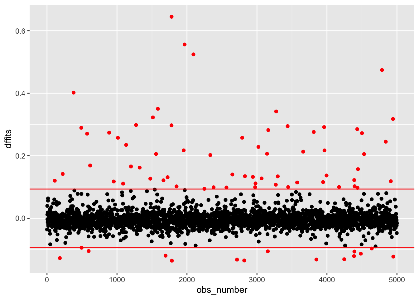
A few points stand out in this plot. We should look into the five points with DFFITS values over 0.4. (Not because 0.4 is a special number, just because it helps us identify those five points.)
Plot the DFBETAS:
library(tidyr)
acs |>
  mutate(obs_number = row_number()) |>
  pivot_longer(cols = starts_with("dfb_") & !ends_with("_large")) |>
  mutate(large = ifelse(abs(value) > 2/sqrt(nobs(mod)),
                        "red", "black")) |>
  ggplot(aes(obs_number, value, color = large)) +
  geom_point() +
  geom_hline(yintercept = c(-1,1) * 2/sqrt(nobs(mod)), color = "red") +
  facet_wrap(~ name) +
  scale_color_identity()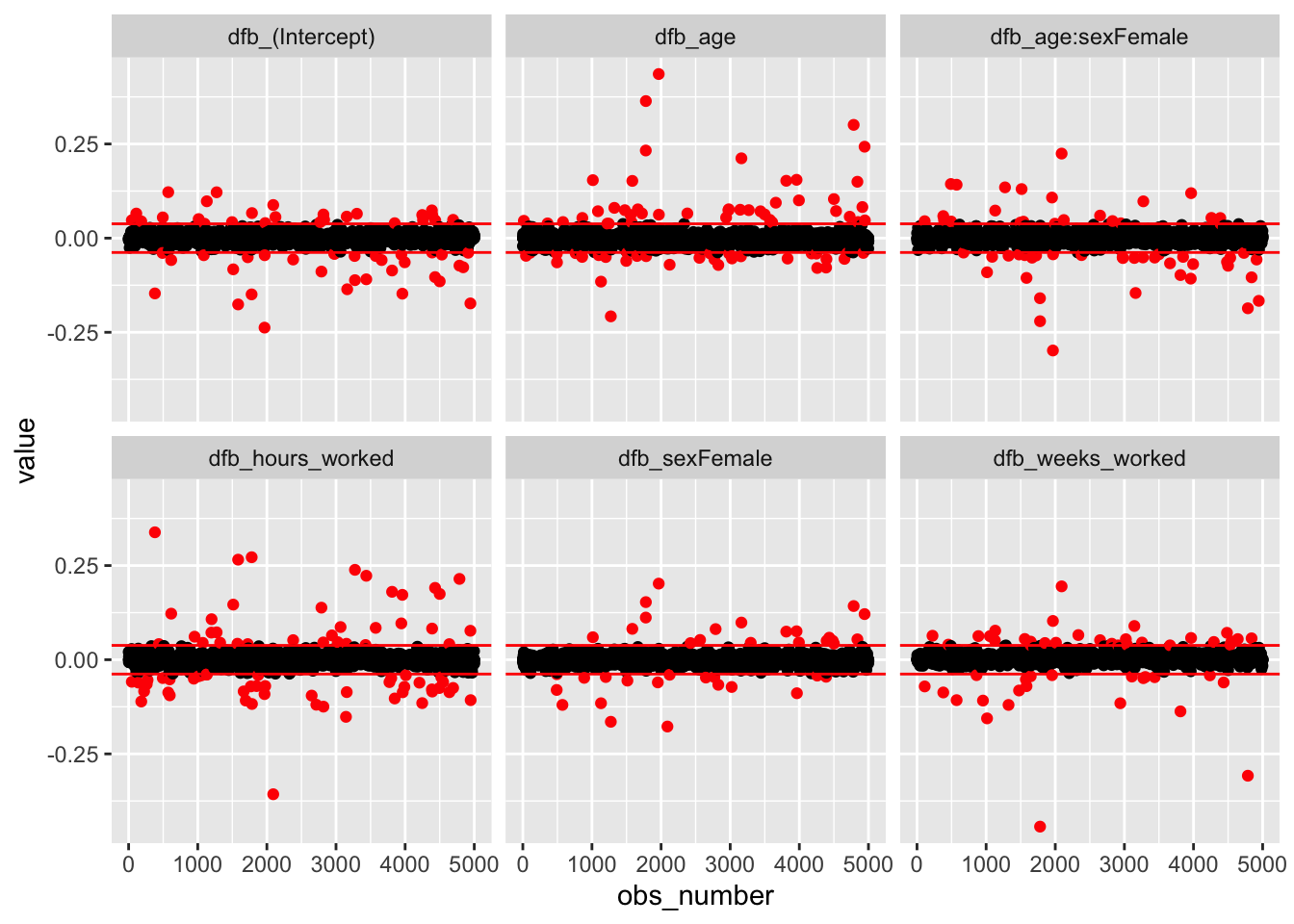
Several points stand out in the plots for age, the interaction of age and sex, hours_worked, and weeks_worked. These plots have a few large positive and/or negative DFBETAS around observations 2000 and 5000.
To investigate any points we identified in the plot, we can take a subset of our data, filtering observations by any cutoffs we decided on after looking at the plots:
influential_obs <-
  acs |>
  filter(dffits > .4 |
           if_any(.cols = starts_with("dfb_") & !ends_with("_large"),
                  .fns = ~ abs(.) > .25))
This subset has only six observations, meaning these points were responsible for influencing the fit and a number of parameters. Of course, we could adjust our cutoffs to identify even more observations we should investigate, but this is a good place to start.
8.4 Corrective Actions
First, investigate why some observations were identified as outliers. Here, subject matter knowledge is crucial. Outlier detection methods simply tell us which observations are different or influential, and our task is to figure out why certain observations are outliers.7
Before you investigate individual observations in-depth, revisit the other assumptions. A violation of another assumption can have the effect that we identify many observations as outliers.
- Examine the dataset.
- Read the codebook and any other associated documentation for the dataset.
- Consider how the data was collected (oral interviews, selected-response surveys, open-response surveys, web scraping, government records, etc.).
- Consider how the population of generalization is defined, and how this sample was drawn.
- For observations identified as having outlying values, check whether they differ from the other observations with respect to other variables.
Then, based on your findings, decide what to do with the outliers.8 Always make a note in your write-up how you handled outliers.
- If you found a pattern in the observations with outliers, modify the model (add, drop, or transform variables). Examples:
- Individuals who reported extremely high values of income also reported working over ninety hours per week, and hours worked was not included as a predictor.
- Individuals who reported extremely long commute times also reported they take ferryboats to work, and mode of transportation was not included in the model.
- If you know (with relative certainty) what the value should be, correct it. Examples:
- Data entry errors like misplaced decimal points (GPA of 32.6 instead of 3.26).
- Incorrect scale of variable (monthly rather than yearly income).
- If the observation is not from the target population, either remove it or adjust your generalizations. Examples:
- Study on trends in teacher use of technology in 2000-2020 includes period of fully-remote learning during pandemic.
- Data used to answer questions about workplace interactions includes individuals working from home.
- If the value reflects construct-irrelevant variance, remove it. Examples:
- An extremely long reaction time in a laboratory task after a participant was distracted by a noise next door.
- Bias or differential item functioning in surveys or assessments.
- If the distribution of values does not match the distribution assumed by the model, modify the model (add, drop, or transform variables) or fit a generalized linear model. Examples:
- Income follows a skewed distribution so a model assuming normality would identify legitimate values as outliers.
- An unmodeled categorical variable causes the outcome (and residuals) to have a bimodal distribution.
Additional recommendations apply to situations using structural equation modeling or multilevel modeling.9
After you have applied any corrections or changed your model in any way, you must re-check this assumption and all of the other assumptions.
The cutoff values in this chapter are based on those found in, Belsley, D. A., Kuh, E., and Welsch, R. E. (1980). Regression Diagnostics: Identifying influential data and sources of collinearity. Wiley. https://doi.org/10.1002/0471725153
For a discussion of alternative cutoffs, see chapter 4 of, Fox, J. D. (2020). Regression diagnostics: An introduction (2nd ed.). SAGE. https://doi.org/10.4135/9781071878651↩︎For examples and discussion, see, Bollen, K. A., & Jackman, R. W. (1985). Regression diagnostics: An expository treatment of outliers and influential cases. Sociological Methods & Research, 13(4), 510-542. https://doi.org/10.1177/0049124185013004004↩︎
For more cases and examples, see chapter seven in, Osborne, J. (2013). Best practices in data cleaning: A complete guide to everything you need to do before and after collecting your data. Sage. https://doi.org/10.4135/9781452269948↩︎
Aguinis, H., Gottfredson, R. K., & Joo, H. (2013). Best-practice recommendations for defining, identifying, and handling outliers. Organizational Research Methods, 16(2), 270-301. http://doi.org/10.1177/1094428112470848↩︎