5 Homoscedasticity

What this assumption means: The residuals have equal variance (homoscedasticity) for every value of the fitted values and of the predictors.

Why it matters: Homoscedasticity is necessary to calculate accurate standard errors for parameter estimates.

How to diagnose violations: Visually check plots of residuals against fitted values or predictors for constant variance, and use the Breusch-Pagan test against heteroscedaticity (non-constant variance).

How to address it: Modify the model, fit a generalized linear model, or run a weighted least squares regression.

5.1 Example Model

If you have not already done so, download the example dataset, read about its variables, and import the dataset into R.

Then, use the code below to fit this page’s example model.

acs <- readRDS("acs2019sample.rds")
mod <- lm(weeks_worked ~ age + hours_worked + commute_time + education, acs, na.action = na.exclude)

5.2 Statistical Tests

Use the Breusch-Pagan test to assess homoscedasticity. The Breusch-Pagan test regresses the residuals on the fitted values or predictors and checks whether they can explain any of the residual variance. A small p-value, then, indicates that residual variance is non-constant (heteroscedastic).

Load the car package to use its Breusch-Pagan test in ncvTest(), where “ncv” stands for “non-constant variance”. The default of ncvTest() is to regress the residuals on the fitted values.

library(car)
ncvTest(mod)

## Non-constant Variance Score Test 
## Variance formula: ~ fitted.values 
## Chisquare = 993.4585, Df = 1, p = < 2.22e-16

The small p-value leads us to reject the null hypothesis of homoscedasticity and infer that the error variance is non-constant.

In the second argument of ncvTest(), we can specify a one-sided formula with one or more variables to test whether the variance is non-constant for these terms.

ncvTest(mod, ~ commute_time)

## Non-constant Variance Score Test 
## Variance formula: ~ commute_time 
## Chisquare = 1.884285, Df = 1, p = 0.16985

ncvTest(mod, ~ age + hours_worked)

## Non-constant Variance Score Test 
## Variance formula: ~ age + hours_worked 
## Chisquare = 910.6193, Df = 2, p = < 2.22e-16

We failed to reject homoscedasticity for commute_time alone, but we would reject it for a combination of age and hours_worked.

5.3 Visual Tests

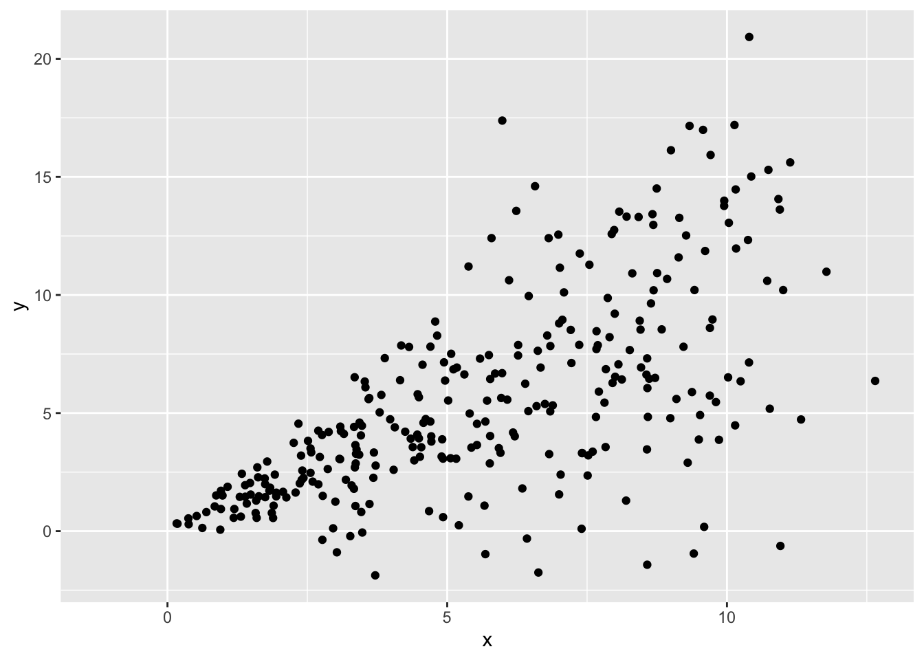
A classic example of heteroscedasticity is a fan shape. We often see this pattern when predicting income by age, or some outcome by time in longitudinal data, where variance increases with our predictor.

Heteroscedasticity can follow other patterns too, such as constantly decreasing variance, or variance that increases then decreases then increases again.

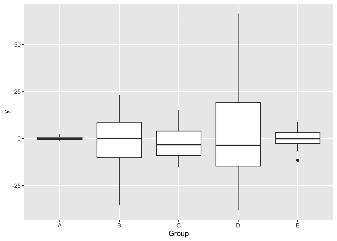
It can also exist when variance is unequal across groups (categorical predictors):

To check the assumption of homoescedasticity visually, first add variables of fitted values and of the square root of the absolute value of the standardized residuals (\(\sqrt{\lvert standardized \; residuals \rvert}\)) to the dataset.

We can then create a scale-location plot, where a violation of homoscedasticity is indicated by a non-flat fitted line. Because we forced all the residuals to be positive by taking their absolute value, instead of looking for whether the band of points is wider or narrow (variance is larger or smaller) at each value of \(x\), we simply look for whether the line goes up or down.

We must plot the residuals against the fitted values and against each of the predictors.

library(dplyr)
acs <-
  acs |> 
  mutate(yhat = fitted(mod),
         res_sqrt = sqrt(abs(rstandard(mod))))

Plot res_sqrt against the fitted values.

The residual variance is decidedly non-constant across the fitted values since the conditional mean line goes up and down, suggesting that the assumption of homoscedasticity has been violated.

library(ggplot2)
ggplot(acs, aes(yhat, res_sqrt)) +
  geom_point() +
  geom_smooth()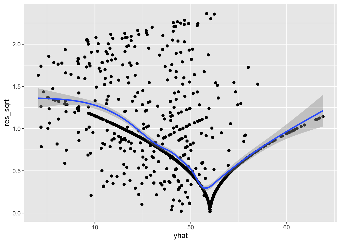

The residual variance is decidedly non-constant across the fitted values since the conditional mean line goes up and down, suggesting that the assumption of homoscedasticity has been violated. This matches the conclusion we would draw from the Breusch-Pagan test earlier.

Check the residuals against each predictor. We will just check commute_time, which had a non-significant p-value in our test earlier.

ggplot(acs, aes(commute_time, res_sqrt)) +
  geom_point() +
  geom_smooth()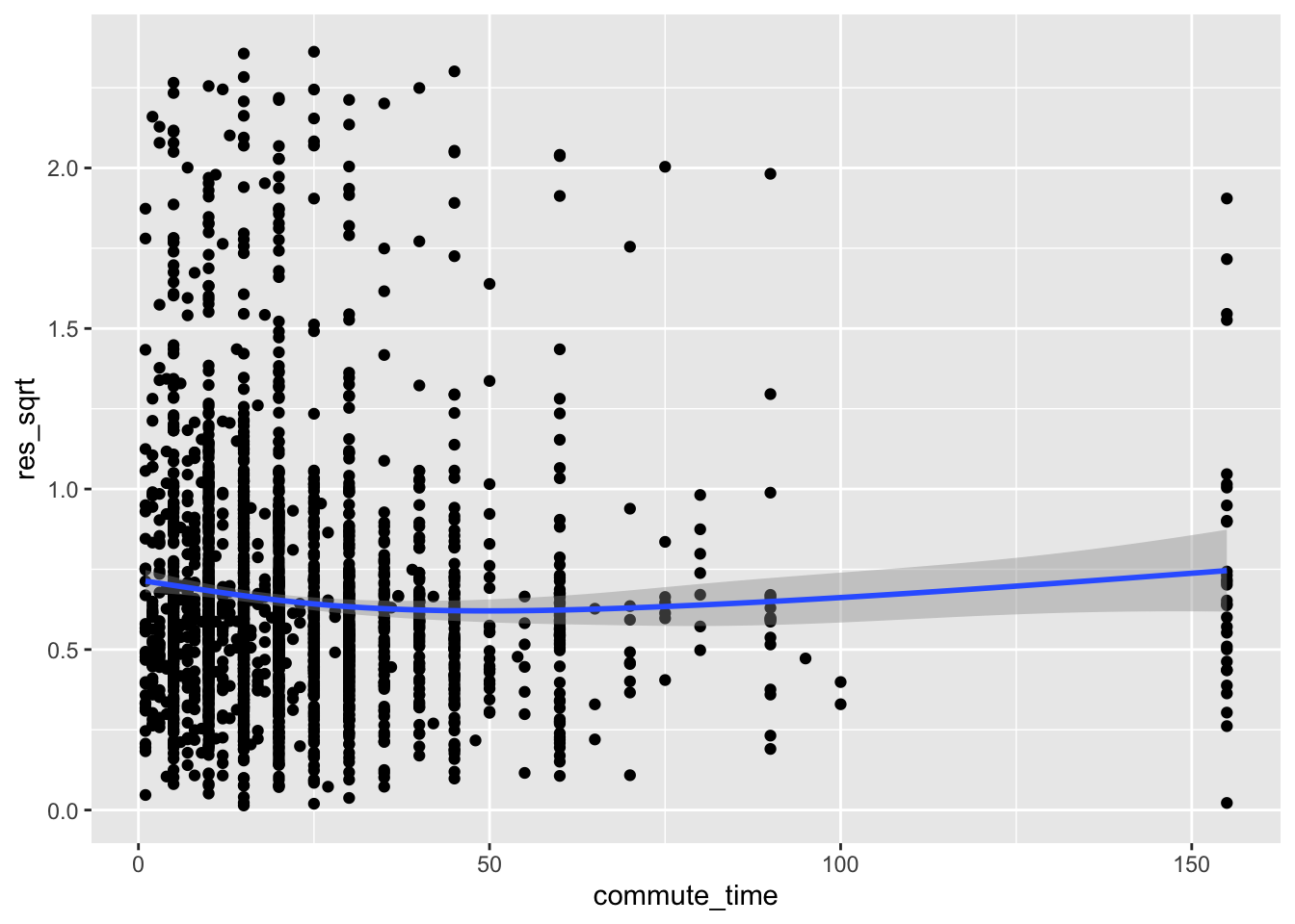

Here, the line is relatively flat, meaning we failed to find evidence of heteroscedasticity. We made the same conclusion earlier with the Breusch-Pagan test where we regressed the residuals on commute_time.

Now, check the residual variance against a categorical predictor, education.

Adding a conditional mean line with a categorical variable requires extra steps in R:

If the categorical variable is a factor, use as.numeric(var) to make it numeric. If it is a character, make it a factor and then numeric with as.numeric(as.factor(var)).
Use stat_summary() with additional arguments, instead of geom_smooth().

ggplot(acs, aes(as.numeric(education), res_sqrt)) + 
  geom_point() +
  stat_summary(geom = "line", fun = mean, color = "blue", size = 1.5)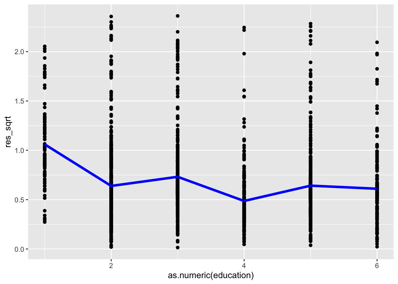

The line is not flat, indicating heteroscedasticity across the levels of education.

5.4 Corrective Actions

To address violations of the assumption of homoscedasticity, try the following:

Check the other regression assumptions, since a violation of one can lead to a violation of another.
Modify the model formula by adding or dropping variables or interaction terms.
Fit a generalized linear model.
Instead of ordinary least squares regression, use weighted least squares.

After you have applied any corrections or changed your model in any way, you must re-check this assumption and all of the other assumptions.