9 Logistic Regression
Logistic regression is used when predicting binary outcomes, such as voting for a certain presidential candidate or answering a test question correctly.
The assumptions of normality and homoscedasticity do not apply to logistic regression, but others do:
And we have a new assumption:
In this chapter, we will learn how to test these assumptions for a logistic regression model.
9.1 Setup
If you have not already done so, download the example dataset, read about its variables, and import the dataset into R.
Then, use the code below to fit this page’s example model.
We will add a new variable, higher_ed_degree, an indicator whether somebody has a bachelor’s or advanced degree.
library(dplyr)
library(ggplot2)
library(tidyr)

acs <-
  readRDS("acs2019sample.rds") |>
  mutate(higher_ed_degree = as.numeric(education %in% c("Bachelor's degree", "Advanced degree")))

mod <-
  glm(higher_ed_degree ~ age + commute_time + weeks_worked + hours_worked,
      acs,
      family = binomial,
      na.action = na.exclude)

summary(mod)
##
## Call:
## glm(formula = higher_ed_degree ~ age + commute_time + weeks_worked +
## hours_worked, family = binomial, data = acs, na.action = na.exclude)
##
## Coefficients:
## Estimate Std. Error z value Pr(>|z|)
## (Intercept) -1.416638 0.274160 -5.167 2.38e-07 ***
## age 0.001241 0.003079 0.403 0.686867
## commute_time 0.001593 0.002032 0.784 0.433011
## weeks_worked -0.001331 0.005134 -0.259 0.795467
## hours_worked 0.012642 0.003824 3.306 0.000946 ***
## ---
## Signif. codes: 0 '***' 0.001 '**' 0.01 '*' 0.05 '.' 0.1 ' ' 1
##
## (Dispersion parameter for binomial family taken to be 1)
##
## Null deviance: 2796.9 on 2315 degrees of freedom
## Residual deviance: 2783.5 on 2311 degrees of freedom
## (2684 observations deleted due to missingness)
## AIC: 2793.5
##
## Number of Fisher Scoring iterations: 49.2 Linearity
In logistic regression (and other generalized linear models, for that matter), the assumption of linearity carries the same basic meaning of correct functional form, the same problems of incorrect specification when it is violated, and the same corrective action of model modification. However, the diagnostic test differs for logistic regression.
In OLS regression, we thought we were checking whether there was a linear relationship between the outcome and the predictors. However, we were actually checking whether there was a linear relationship on the link scale. OLS regression uses the identity link, where variables are not transformed, so we could ignore this qualification. When we use a different link, we must adapt our tests.
In logistic regression, we assume the relationship is linear on the logit scale. This is assessed with component-plus-residual plots. The “component” is the values of a variable multiplied by its estimated coefficient (meaning that each predictor has its own component vector), and the “residual” is the working residuals, a type of residuals in generalized linear models.
9.2.1 Visual Tests
To diagnose violations of linearity, we plot each predictor against its component-plus-residual.
We will add a variable called comp_res with the values of weeks_worked multiplied by its coefficient, plus the working residuals. (Afterward, we should repeat this process with the other predictors. Note that the variable needs to be specified a three points: twice within mutate() and once within the aes() call of ggplot().)
In our plot, we add a dashed red line that is a linear fit of the points, and a blue smoothed conditional mean line. If a linear fit is appropriate, the two lines will be close to each other. Note that the “goal” line is not horizontal at zero as it was in OLS regression.
acs |>
  mutate(comp_res = coef(mod)["commute_time"]*commute_time + residuals(mod, type = "working")) |>
  ggplot(aes(x = commute_time, y = comp_res)) +
  geom_point() +
  geom_smooth(color = "red", method = "lm", linetype = 2, se = F) +
  geom_smooth(se = F)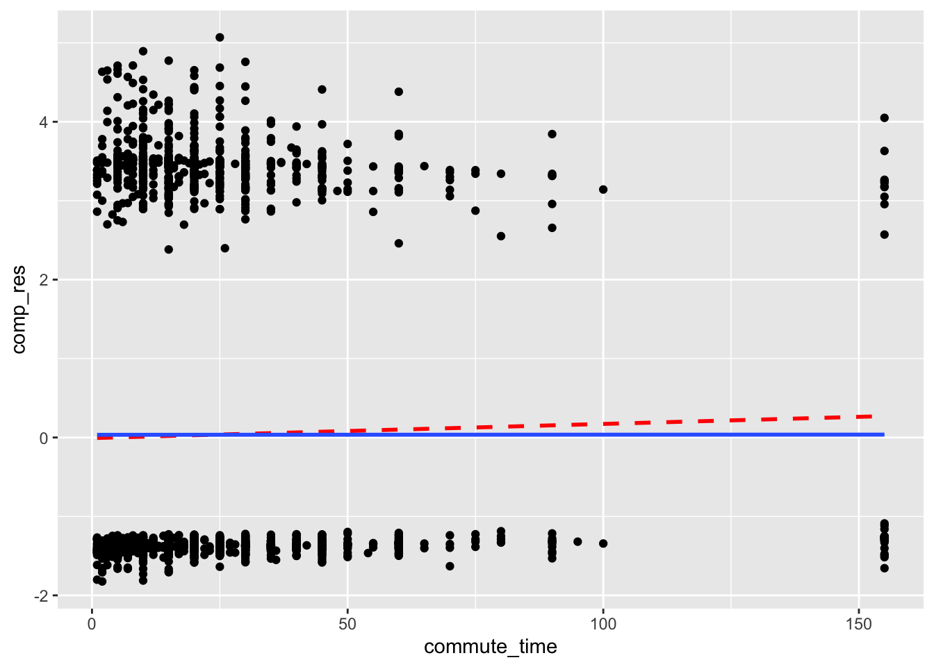
The two lines are close to each other, so there is no concern arising from the commute_time variable.
Now let’s look at the component-plus-residual plot for age:
acs |>
  mutate(comp_res = coef(mod)["age"]*age + residuals(mod, type = "working")) |>
  ggplot(aes(x = age, y = comp_res)) +
  geom_point() +
  geom_smooth(color = "red", method = "lm", linetype = 2, se = F) +
  geom_smooth(se = F)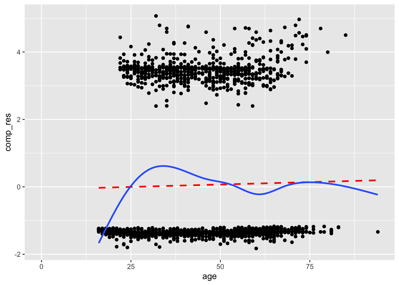
The systematic rise then fall in the smoothed line suggests a nonlinear relationship for age. The model estimates suggest a constant increase in the likelihood of a higher education degree with age, but the data suggests that the likelihood increases and then decreases.
Adding a term for age squared improves the component-plus-residual plot, although we should still be a little concerned about the rise of the smoothed line on the right side of the plot.
Notice how the model estimates show a negative quadratic term for age.
mod2 <-
  glm(higher_ed_degree ~ age + I(age^2) + commute_time + hours_worked + sex,
      acs,
      family = binomial,
      na.action = na.exclude)

summary(mod2)
##
## Call:
## glm(formula = higher_ed_degree ~ age + I(age^2) + commute_time +
## hours_worked + sex, family = binomial, data = acs, na.action = na.exclude)
##
## Coefficients:
## Estimate Std. Error z value Pr(>|z|)
## (Intercept) -4.2661525 0.4452196 -9.582 < 2e-16 ***
## age 0.1337058 0.0221577 6.034 1.60e-09 ***
## I(age^2) -0.0015146 0.0002516 -6.020 1.75e-09 ***
## commute_time 0.0016350 0.0020903 0.782 0.4341
## hours_worked 0.0103158 0.0040751 2.531 0.0114 *
## sexFemale 0.6165557 0.0967227 6.374 1.84e-10 ***
## ---
## Signif. codes: 0 '***' 0.001 '**' 0.01 '*' 0.05 '.' 0.1 ' ' 1
##
## (Dispersion parameter for binomial family taken to be 1)
##
## Null deviance: 2796.9 on 2315 degrees of freedom
## Residual deviance: 2694.5 on 2310 degrees of freedom
## (2684 observations deleted due to missingness)
## AIC: 2706.5
##
## Number of Fisher Scoring iterations: 4acs |>
mutate(comp_res = coef(mod2)["age"]*age + residuals(mod2, type = "working")) |>
ggplot(aes(x = age, y = comp_res)) +
geom_point() +
geom_smooth(color = "red", method = "lm", linetype = 2, se = F) +
geom_smooth(se = F)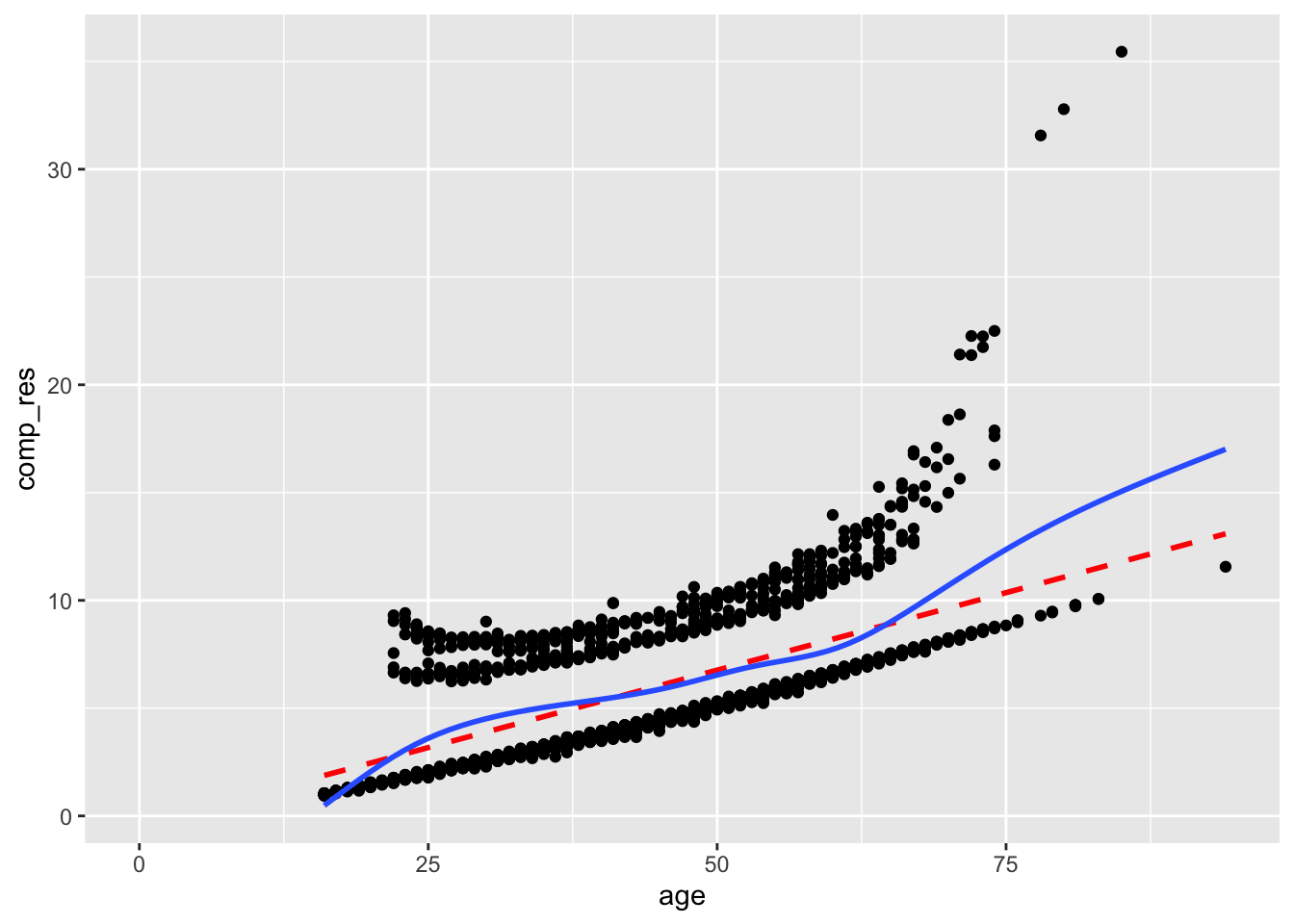
See the chapter on Linearity for more guidance on corrective actions.
9.3 Independence
The questions we ask in logistic regression are the same as those we ask in OLS regression. See the chapter on Independence.
9.4 No Multicollinearity
In OLS regression, multicollinearity can be calculated either from the correlations among the predictors, or from the correlations among the coefficient estimates, and these result in the same variance inflaction factors (VIFs).
In GLMs, these two approaches yield similar but different VIFs. John Fox, one of the authors of the car package where the vif() function is found, opts for calculating the VIFs from the coefficient estimates.
library(car)
vif(mod)
## age commute_time weeks_worked hours_worked
## 1.012627 1.007908 1.144947 1.142440If we wanted to calculate the VIFs from the correlations among the predictors, all we would have to do is fit a new linear model with lm() and the same outcome and predictors, and then run vif() on that fitted model.
mod_lm <-
  lm(higher_ed_degree ~ age + commute_time + weeks_worked + hours_worked,
     acs,
     na.action = na.exclude)

vif(mod_lm)
## age commute_time weeks_worked hours_worked
## 1.014146 1.009037 1.162936 1.160560Either approach is acceptable since the resulting VIFs are often very similar, and we are not strictly applying any hard cutoffs. None of the VIFs are of a concerning magnitude.
See the chapter on No Multicollinearity for guidance on possible cutoff values for VIFs, issues of polynomials and interactions, and corrective actions.
9.5 No Outlier Effects
We can use DFFITS and DFBETAS to detect influential observations. These are standardized measures of how our model estimates would change had we excluded a given observation. Each observation has one DFFITS, measuring how much prediction for that point would change, and one DFBETAS for each predictor, measuring how much each coefficient would change.
Plot DFFITS and DFBETAS, and look for any noteworthy points or groups of points.
DFFITS:
acs <-
  acs |>
  mutate(dffits = dffits(mod))

acs |>
  mutate(obs_number = row_number(),
         large = ifelse(abs(dffits) > 2*sqrt(length(coef(mod))/nobs(mod)),
                        "red", "black")) |>
  ggplot(aes(obs_number, dffits, color = large)) +
  geom_point() +
  geom_hline(yintercept = c(-1,1) * 2*sqrt(length(coef(mod))/nobs(mod)), color = "red") +
  scale_color_identity()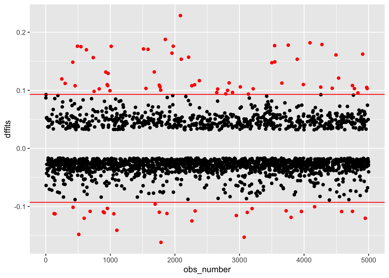
DFBETAS:
acs <-
  dfbetas(mod) |>
  as.data.frame() |>
  rename_with(~ paste0("dfb_", .x)) |>
  cbind(acs)

acs |>
  mutate(obs_number = row_number()) |>
  pivot_longer(cols = starts_with("dfb")) |>
  mutate(large = ifelse(abs(value) > 2/sqrt(nobs(mod)),
                        "red", "black")) |>
  ggplot(aes(obs_number, value, color = large)) +
  geom_point() +
  geom_hline(yintercept = c(-1,1) * 2/sqrt(nobs(mod)), color = "red") +
  facet_wrap(~ name) +
  scale_color_identity()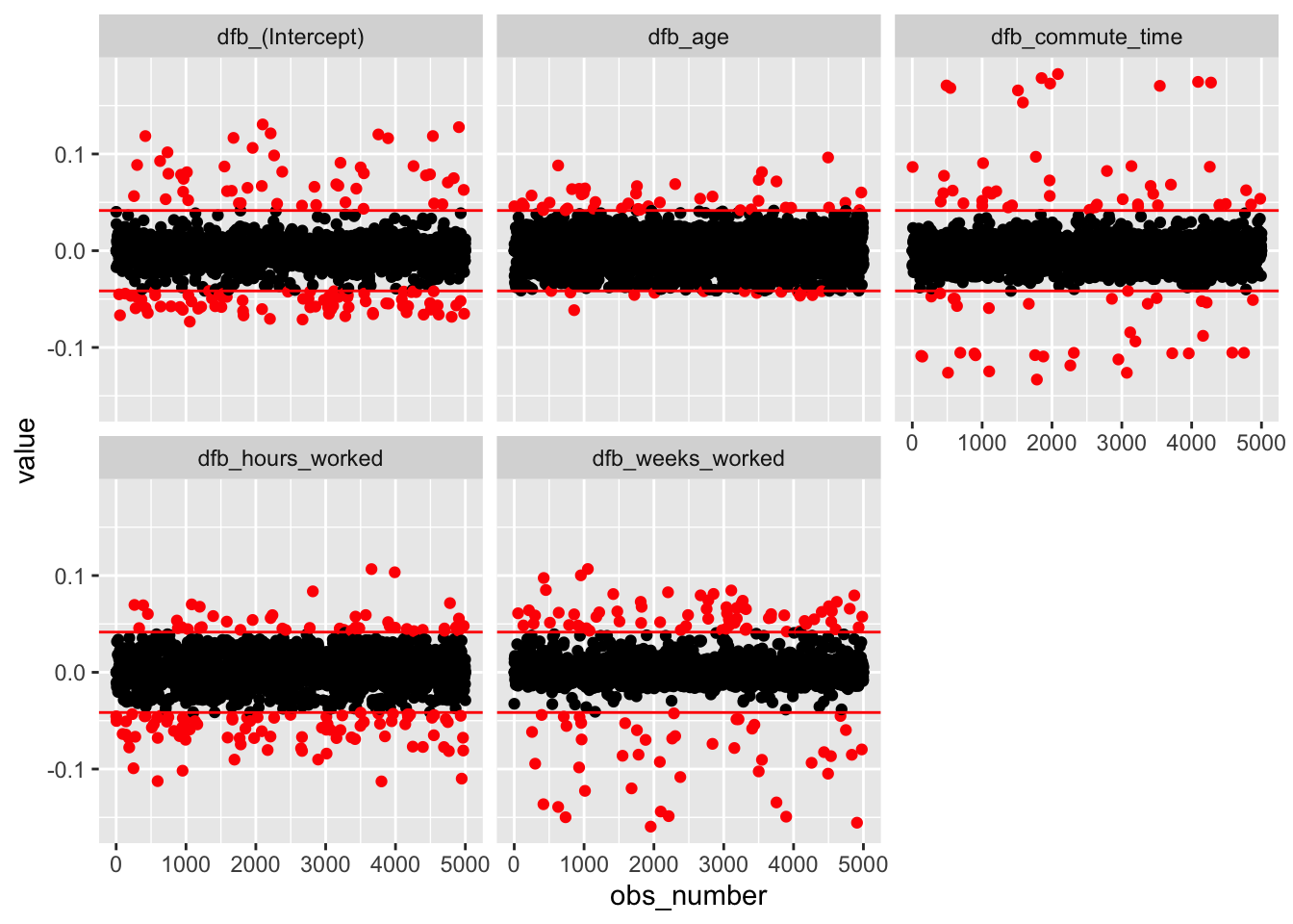
None of these plots show any cause for concern.
See chapter on No Outlier Effects for guidance on corrective actions.
9.6 Fully Represented Data Matrix
What this assumption means: Both levels of the outcome are observed at each level of the predictors.
Why it matters: Very large coefficients due to empty cells in interaction terms.
How to diagnose violations: Make cross-tabulations of categorical predictors and the outcome to check if any cells are empty or have very few cases.
How to address it: Collapse categories of problem variables. Change model to not include variables.
9.6.1 Contingency Tables
An obvious violation of this would occur if we wanted to predict whether a student would receive a passing grade in a class from whether they are right-handed or left-handed, and our data looked like this:
| Fail | Pass | |
| Right-handed | 12 | 0 |
| Left-handed | 1 | 3 |
We cannot estimate the probability that a right-handed student would pass the class, since none did!
It is less obvious when empty cells occur in higher dimensions, and this can happen in models with interaction terms.
Consider a model where we want to predict whether somebody has a higher education degree from their self-rated English language proficiency, marital status, and the interaction of these two variables.
The contingency tables of either variable with higher_ed_degree show a nonzero value in each cell.
with(acs, table(english, higher_ed_degree))## higher_ed_degree
## english 0 1
## Very well 150 43
## Well 41 8
## Not well 28 2
## Not at all 8 1with(acs, table(marital_status, higher_ed_degree))## higher_ed_degree
## marital_status 0 1
## Married 1621 714
## Widowed 235 30
## Divorced 357 93
## Separated 22 2
## Never married 1750 176(Side note: the low cell counts will lead to large standard errors since we can have little confidence where there is little data.)
However, the three-way contingency table reveals a number of empty cells:
with(acs, table(english, marital_status, higher_ed_degree))## , , higher_ed_degree = 0
##
## marital_status
## english Married Widowed Divorced Separated Never married
## Very well 45 4 9 2 90
## Well 18 2 1 2 18
## Not well 12 2 5 0 9
## Not at all 4 2 0 0 2
##
## , , higher_ed_degree = 1
##
## marital_status
## english Married Widowed Divorced Separated Never married
## Very well 29 0 3 0 11
## Well 5 1 1 0 1
## Not well 0 0 1 0 1
## Not at all 0 0 0 0 1Now fit a model with these two variables and their interaction as predictors.
mod_sparse <-
  glm(higher_ed_degree ~ english*marital_status,
      acs,
      family = binomial,
      na.action = na.exclude)

summary(mod_sparse)
##
## Call:
## glm(formula = higher_ed_degree ~ english * marital_status, family = binomial,
## data = acs, na.action = na.exclude)
##
## Coefficients: (3 not defined because of singularities)
## Estimate Std. Error z value Pr(>|z|)
## (Intercept) -0.43937 0.23813 -1.845 0.065 .
## englishWell -0.84157 0.55880 -1.506 0.132
## englishNot well -17.12670 1142.05091 -0.015 0.988
## englishNot at all -17.12670 1978.09018 -0.009 0.993
## marital_statusWidowed -17.12670 1978.09017 -0.009 0.993
## marital_statusDivorced -0.65925 0.70792 -0.931 0.352
## marital_statusSeparated -17.12670 2797.44195 -0.006 0.995
## marital_statusNever married -1.66255 0.39840 -4.173 3.01e-05 ***
## englishWell:marital_statusWidowed 17.71449 1978.09062 0.009 0.993
## englishNot well:marital_statusWidowed 17.12670 3611.48202 0.005 0.996
## englishNot at all:marital_statusWidowed 17.12670 3956.18033 0.004 0.997
## englishWell:marital_statusDivorced 1.94018 1.66033 1.169 0.243
## englishNot well:marital_statusDivorced 16.61588 1142.05163 0.015 0.988
## englishNot at all:marital_statusDivorced NA NA NA NA
## englishWell:marital_statusSeparated 0.84157 3956.18037 0.000 1.000
## englishNot well:marital_statusSeparated NA NA NA NA
## englishNot at all:marital_statusSeparated NA NA NA NA
## englishWell:marital_statusNever married 0.05311 1.21237 0.044 0.965
## englishNot well:marital_statusNever married 17.03139 1142.05144 0.015 0.988
## englishNot at all:marital_statusNever married 18.53547 1978.09058 0.009 0.993
## ---
## Signif. codes: 0 '***' 0.001 '**' 0.01 '*' 0.05 '.' 0.1 ' ' 1
##
## (Dispersion parameter for binomial family taken to be 1)
##
## Null deviance: 275.02 on 280 degrees of freedom
## Residual deviance: 236.37 on 264 degrees of freedom
## (4719 observations deleted due to missingness)
## AIC: 270.37
##
## Number of Fisher Scoring iterations: 16Three problems are apparent:
- Some coefficients are missing.
- Some standard errors are massive.
- Some coefficients are also massive.
On the third point, a coefficient of 17 may not seem very large, but remember that these are log odds ratios. That coefficient means the odds are multiplied by \(e^{17} = 24,154,953\), and in the case of a coefficient estimate of -17, we would divide the odds by that amount.
A related issue is perfect prediction, which can happen with one or more continuous or categorical predictors. In this case, the outcome is fully explained. Similar problems with large coefficient estimates occur.
Create a new variable called adult that is an indicator whether an individual’s age is at least 18. Then, predict adult from age.
acs <-
  acs |>
  mutate(adult = ifelse(age >= 18, 1, 0))

mod_perfect <-
  glm(adult ~ age, acs, family = binomial)

summary(mod_perfect)
##
## Call:
## glm(formula = adult ~ age, family = binomial, data = acs)
##
## Coefficients:
## Estimate Std. Error z value Pr(>|z|)
## (Intercept) -581.04 7596.64 -0.076 0.939
## age 33.21 433.97 0.077 0.939
##
## (Dispersion parameter for binomial family taken to be 1)
##
## Null deviance: 4.9509e+03 on 4999 degrees of freedom
## Residual deviance: 1.5628e-05 on 4998 degrees of freedom
## AIC: 4
##
## Number of Fisher Scoring iterations: 25age has a very large coefficient estimate and standard error.
9.6.2 Corrective Actions
In cases of sparse data or perfect prediction, corrective actions include
- Collect more data. While not always possible, collecting more data can help fill out the data matrix, especially if sampling is targeted at specific subpopulations.
- Collapse categories. Reduce the number of levels in categorical predictors to that no cells in the contingency table are empty.
- Drop variables. Every dataset and each analysis has its limitations, and it is sometimes a fact that the data cannot support the inclusion of one or more variables in a model. You may also want to revisit the model form and critically assess whether it is sensible to predict a given outcome from a given predictor, to give a theoretical justification for not including some variable in the model.