4 Model Specification
To get a sense of MPlus' model specification algebra, as well as some of it's default model assumptions, we will continue to use the data in ex3.1.dat. For this, we can drop the ANALYSIS: command (we will be using the default analysis options), and add a MODEL: command.
4.1 Model Elements
A structural equation model might contain any of the following elements:
- observed (manifest) variables, from your data
- latent (unobserved) variables
- regression (generalized linear) relationships
- measurement relationships, for indicators of latent variables
- variances of exogenous variables
- residual variances of endogenous variables
- covariances, either among exogenous variables or among residuals
- means (intercepts, thresholds, cutpoints)
Observed variables are named on the VARIABLE: command, before they appear in a MODEL:
The key words used in model specification are:
- ON denotes a regression
- BY denotes a measurement
- WITH denotes a covariance
- a variable name (alone) might denote either a variance or a residual variance
- a variable name in square brackets denotes a mean
4.1.1 Regression
A simple regression is specified like this:
title: Simple regression
data:  file=ex3.1.dat;
variable: names= x1 x2 x3;
model:
    x1 on x2 x3;
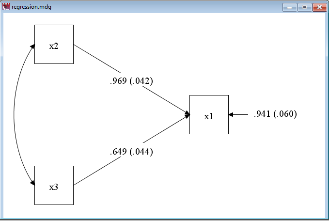
and a portion of our output, the parameter estimates, is:
MODEL RESULTS
                                                    Two-Tailed
                    Estimate       S.E.  Est./S.E.    P-Value
 X1       ON
    X2                 0.969      0.042     23.356      0.000
    X3                 0.649      0.044     14.626      0.000
 Intercepts
    X1                 0.511      0.043     11.765      0.000
 Residual Variances
    X1                 0.941      0.060     15.811      0.000
To use categorical variables as independent (exogenous) variables in any model you have to create indicators (sets of binary variables). You could either include indicators in your input data set, or use the DEFINE: command to create them after the data is read.
Notice (by looking at the full output, not included here) that the default analysis is maximum likelihood estimation, not least squares.
4.1.2 Explicit Covariance
Notice also (by looking at the MPlus diagram, using Alt-D) that this model includes a correlation between x2 and x3, but does not report this in the Model Results. To see a fuller specification of the very same model, try:
title: Simple regression, explicit corr
data:  file=ex3.1.dat;
variable: names= x1 x2 x3;
model:
    x1 on x2 x3;
    x2 with x3;
4.2 Latent Variable Measurement
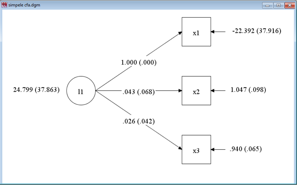
Another key operator is BY, which defines the measurement model elements for a latent variable. This is like a regression path with the restriction that the independent variable must be a latent variable. This is also known as confirmatory factor analysis.
As a bad example (but using the same data), look at:
title: Simple CFA
data:  file=ex3.1.dat;
variable: names= x1 x2 x3;
model:
    L1 by x1 x2 x3;
Here, L1 is a latent variable, not part of the input file and *not named in the VARIABLE: section. By default, the measurement path from L1 to x1 (the first variable encountered in the BY list) is fixed at 1 (one). Also by default, there are no correlations among the residual variances for x1, x2, and x3.
 (To see why this is such a poorly fitting model, look at the correlation matrix from the sample statistics, in Chapter 3. The very low correlation between x2 and x3 is not consistent with the other correlations.)
4.3 Fixing and Freeing Parameters
Model constraints are required to identify (fix a measurement scale) latent variables. Constraints are also useful for specifying some models. Constraints come in three fundamental varieties:
fixing and freeing parameters, and equality constraints. Parameters are fixed at a particular value with @, and freed with an asterisk, *.
4.3.1 Fixing a Covariance
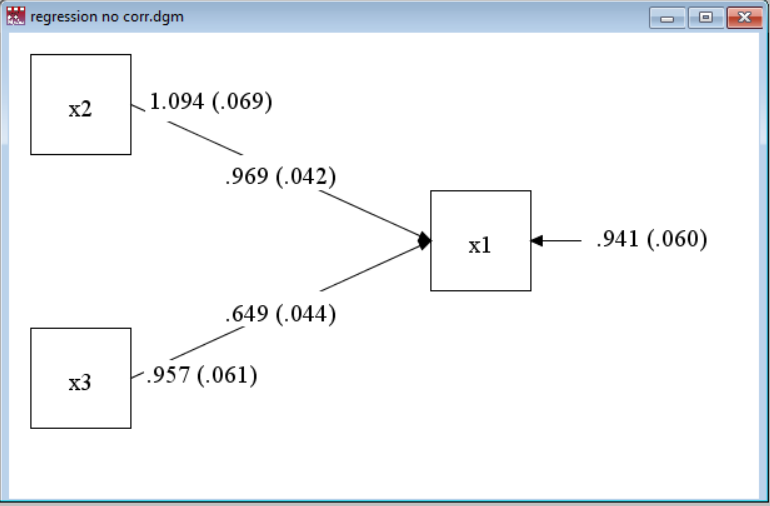
Going back to the regression example above, a modification we can make to that model is to specify that x2 and x3 have no (that is, zero) correlation. Try:
title: Simple regression, no corr
data:  file=ex3.1.dat;
variable: names= x1 x2 x3;
model:
    x1 on x2 x3;
    x2 with x3 @0;
(The lack of change in the parameters from the default model with an exogenous covariance reinforces the notion that the exogenous covariance was essentially zero.)
4.3.2 Fixing a Measurement Scale
For example, we could change the scaling variable from x1 to x2 by reordering the variables in the model command (this is typical style), or we could explictly free x1 and fix x2 @1.
title: Simple CFA, scale by x2
data:  file=ex3.1.dat;
variable: names= x1 x2 x3;
model:
    L1 by x1* x2@1 x3;
4.3.3 Standardizing a Latent Variable
So far, we have left means and variances to be freely estimated, but we can constrain these as well. In the modeling algebra here, variances are specified by simply naming each variable, while means are specified by putting a variable name in square brackets.
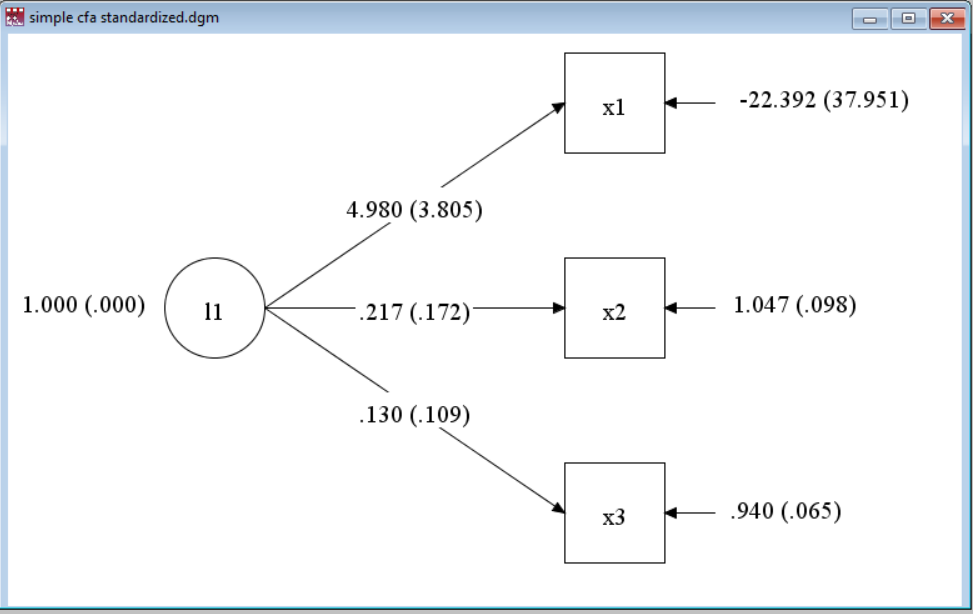
For example, if we specify our latent variable to have a mean of zero (which is the default) and a variance of 1 (one), we specify:
title: Simple CFA, standardized latent var
data:  file=ex3.1.dat;
variable: names= x1 x2 x3;
model:
    L1 by x1* x2 x3;
    L1@1;    ! variance fixed to 1;
    [L1@0];  ! mean fixed to 0;
(Note in the usual version of this model, we free x1, otherwise it is fixed to 1 by default. This model still fits poorly, for the same reason as before.)

4.4 More
As we work our way into more complicated types of models - multilevel, latent class - we will encounter other model operators.