9 Grouped Analysis
So far in our examination of simple SEM models, we have managed to avoid consideration of independent (exogenous) variables that are categorical. There are two different uses that we will consider here, exogenous indicator variables, and grouped analysis. (A third approach, random effects, will be considered later.)
9.1 Grouped Variances-Means Models
9.1.1 Everything is Free
The default with no model command is:
title: CFA grouped variance-means
data: file = ex5.15.dat;
variable: names = y1-y6 x1-x3 g;
            usevariables = y1-y3 g;
grouping = g (1=group1 2=group2);9.1.2 Equal means
If we include a model command, and explicitly ask for a variance-means model, we have all means equal by default. See the scalar measurement model, below.
This will be typical as we examine more complicated models: the overall model command assume equal means and measurement paths, but not variances or residual variances.
title: Group variance-means, means equal
data: file = ex5.15.dat;
variable: names = y1-y6 x1-x3 g;
            usevariables = y1-y3 g;
            grouping = g (1=group1 2=group2);
model:
    y1 - y3;
[y1 - y3];9.1.3 Freeing Default Constraints
To get back to our first model, we can begin with the second specification and add a submodel that frees the means in the submodeled group. Since we only have two groups here, we could specify either one.
title: Group variance-means, constraint freed
data: file = ex5.15.dat;
variable: names = y1-y6 x1-x3 g;
            usevariables = y1-y3 g;
            grouping = g (1=group1 2=group2);
model:
    y1 - y3;
    [y1 - y3];

    model group1:
[y1 - y3];From this point, add constraints across parameters within groups works as it did before, in single group analysis.
9.2 Grouped Regression Models
9.2.1 Default grouped regression
The default model imposes no equality constraints, in contrast to the variances-means model and in contrast to the confirmatory factor. It is very similar to a regression model with a factor variables and all interactions against that factor. The one major difference is that this model does not assume there is a single residual variance term.
title: Grouped regression
data: file = ex5.15.dat;
variable: names = y1-y6 x1-x3 g;
            usevariables = y1-y3 g;
            grouping = g (1=group1 2=group2);
model:
    y1 on y2 y3;
!no cross-group constraints;9.2.2 Constraints for Simple Additive Regression
We can specify constraints on the overall model that turn this back into a simple, additive regression, with a single residual term.
title: Grouped regression, additive
data: file = ex5.15.dat;
variable: names = y1-y6 x1-x3 g;
            usevariables = y1-y3 g;
            grouping = g (1=group1 2=group2);
model:
    y1 on y2 y3 (a b); ! regression paths equal;
y1 (c); ! single residual;If we define a new variable \(xg = g - 1\), then this could also be specified as the single-group model
model: y1 on y2 y3 xg;9.3 Grouped Confirmatory Factor Analysis
Consider a confirmatory factor analysis for two groups. We might wonder if the mean factor score was different between the two groups. First, however, we ought to wonder whether our measurement model is measuring the same thing in both groups. Assessing cross-group invariance requires more complicated modeling than simply assuming it. However, MPlus makes several common sets of restriction very easy to specify.
Grouped analysis, specifying sub-models with the same types of relationships in different sub-populations, is set up via the grouping option of the variables: command.
title: CFA grouped
data: file = ex5.15.dat;
variable: names = y1-y6 x1-x3 g;
            usevariables = y1-y3 g;
            grouping = g (1=group1 2=group2);
model:  f1 by y1-y3;
It is recommended that you give your groups labels, otherwise specify a number of groups (n) and MPlus supplies default group labels (g1 through gn).
9.3.1 Regular Invariance Models
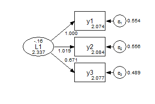
The default model is a scalar model, one in which we assume that measurement paths and measurement intercepts are equal across groups (but not necessarily tau-equivalent). Note that factor means are free to vary. To identify the model, the first factor mean is fixed at zero, and the first measurement paths are fixed at one.
Group 1 Scalar 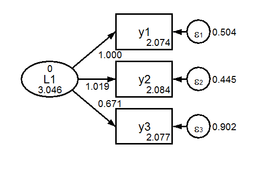 Group 2 Scalar
We can also easily ask MPlus to estimate and compare three different models with different commonly used constraints: the default scalar model, a metric model, and a configural model. (A downside of asking for more than one is that you no longer get a diagram.)
title: CFA grouped
data: file = ex5.15.dat;
variable: names = y1-y6 x1-x3 g;
            usevariables = y1-y3 g;
            grouping = g (1=group1 2=group2);
analysis: model = configural metric scalar;
    ! ask for any combination of these three;
model: f1 by y1-y3;In the configural model, the only constraints are the identifying constraints that the factor means are zero and the first measurement path is fixed at one. Everything else is free to vary between the groups.
Group 1 Configural 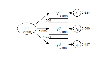
Group 2 Configural 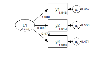
In the metric model, the measurement paths are constrained across groups, and the factor means are fixed at zero.
Group 1 Metric 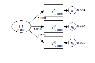
Group 2 Metric 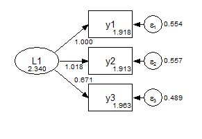
Formal model comparison is given in the first part of the output:
MODEL FIT INFORMATION
Invariance Testing
                   Number of                   Degrees of
     Model        Parameters      Chi-square    Freedom     P-value
     Configural        18              0.000         0       0.0000
     Metric            16            255.148         2       0.0000
     Scalar            14            255.383         4       0.0000
                                               Degrees of
     Models Compared              Chi-square    Freedom     P-value
     Metric against Configural       255.148         2       0.0000
     Scalar against Configural       255.383         4       0.0000
     Scalar against Metric             0.235         2       0.8892
Finally, we can consider a further set of constraints for a strongly invariant model, where the only parameter that varies across groups is the factor mean.
title: CFA grouped, strong invariance
data: file = ex5.15.dat;
variable: names = y1-y6 x1-x3 g;
            usevariables = y1-y3 g;
            grouping = g (1=group1 2=group2);
model: f1 by y1-y3; ! do not vary across groups by default;
        f1 (1);      ! constrained to not vary across groups;
        ![y1-y3];    ! do not vary across groups by default;
y1-y3 (2-4); ! constrained to not vary across groups;Group 1 Strong Invariance 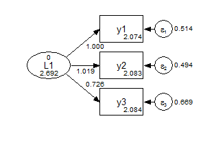
Group 2 Strong Invariance 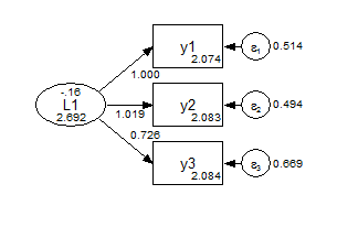
This is equivalent to using the grouping variable as an exogenous covariate.
title: CFA with binary ex
data: file = ex5.15.dat;
variable: names = y1-y6 x1-x3 g;
            usevariables = y1-y3 xg;
define: xg = g - 1;
model:  f1 by y1-y3;
f1 on xg;Group as an exogenous variable 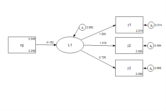
9.3.2 Partial Invariance
Use a metric model, and allow y3 to vary across groups. Or use a scalar model, and allow y3 and [y3] to vary.
title: Partial invariance
data: file = ex5.15.dat;
variable: names = y1 - y6 x1-x3 g;
    usevariables y1 - y3 g;
    grouping = g (1=group1 2=group2);
model:
    L1 by y1 - y3; !scalar default;

    model group2:
    L1 by y3;   !free path;
    [y3];       !free intercept;
9.3.3 Multivariate Models
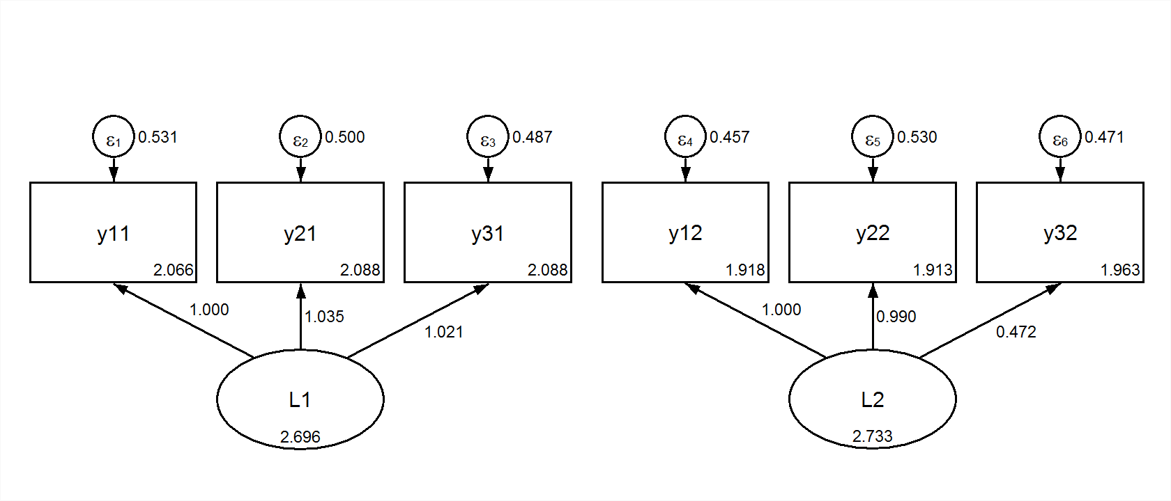
We could reshape the data to wide form. Then, using full-information maximum likelihood we could fit the same two group model in wide (multivariate) form. This is the configural model:
title: Multivariate Congruent
data: file = ex5.15.csv;
    data longtowide:
        long=y1|y2|y3 ;
        wide= y11 y12 | y21 y22| y31 y32  ;
        idvariable=gobs;
        repetition=g (1-2); !specify values if not 0 to n;
variable: names = y1 - y3 g gobs;
    usevariables y11 y21 y31 y12 y22 y32;
model:
    L1 by y11 y21 y31;
    L2 by y12 y22 y32;