4.5 Dropping unneeded observations

SSCC - Social Science Computing Cooperative

Supporting Statistical Analysis for Research

4.5.1 Data concepts - Conditionally dropping observations

Observations are typically dropped based on a variable having a specific condition. For example in a large data set that contains city-level information from Wisconsin, we may only be interested in the cities in Dane county. We could drop all observations that do not contain Dane in a variable that records the county for the observation. Note, this approach differs from how variables are typically excluded from a data set, which is by name or position.

To drop observations, you will need to understand how to test for a condition and how to apply the test to all observations. These topics are covered in the remainder of this section.

4.5.2 Programming skills

4.5.2.1 Conditional tests

A conditional test compares two values. How the two values are compared is determined by the comparison operator used. There are a number of comparisons and the following is a list of the common comparison operators that are used in R and Python.

	operator	usage	comparison
1	==	x == y	equality
2	!=	x != y	not equal
3	>	x > y	x greater than y
4	>=	x >= y	x greater than or equal to y
5	<	x < y	x less than y
6	<=	x <= y	x less than or equal to y

The results of a conditional test is a boolean value (true or false) or possibly the missing value indicator.

The above comparison operators can be combined with the following logical operators to check for more complicated conditions. These logical operations also result in a boolean value or the missing indicator.

	R operator	Python operator	Operation	Condition for result of true
1	&	and	logical and	both the left and right must be true
2	\|	or	logical or	either the left or right must be true
3	!	not	logical complement	the right value must be false

4.5.2.2 Array programming

Array programming allows the application of an operation to be applied to a set of values. Array programming is used by both R and Python to operate on all elements of a data frame variable with one function/method call. In this context array programming is often called vectorized operations.

In this section we will use vectorization to determine which observations to drop, by applying a conditional test to all rows of a variable. This is visualized in figure 4.2. Each of the n values of the vector being tested are checked using the specified condition. The result is a variable that contains n boolean values which indicate if the condition was true or false for each row of the variable. The conditional results variable can now be used to determine which rows to drop or retain (using inclusion or exclusion.) Note, the condition result variable does not need to be saved as a variable of the data frame, although it can be.

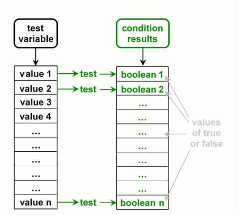
Figure 4.2: Column index of a data frame

4.5.3 Examples - R

These examples use the airAccs.csv data set.

We begin by using the same code as in the prior sections of this chapter to load the tidyverse, import the csv file, and rename the variables.

airAccs_path <- file.path("..", "datasets", "airAccs.csv")
air_accidents_in <- read_csv(airAccs_path, col_types = cols())

Warning: Missing column names filled in: 'X1' [1]

air_accidents_in <-
  rename(
    air_accidents_in,
    obs_num = 1,
    date = Date,
    plane_type = planeType,
    dead = Dead,
    aboard = Aboard,
    ground = Ground
    )

air_accidents <-
  air_accidents_in %>%
  select(-obs_num)

glimpse(air_accidents)

Observations: 5,666
Variables: 7
$ date       <date> 1908-09-17, 1912-07-12, 1913-08-06, 1913-09-09, 19...
$ location   <chr> "Fort Myer, Virginia", "Atlantic City, New Jersey",...
$ operator   <chr> "Military - U.S. Army", "Military - U.S. Navy", "Pr...
$ plane_type <chr> "Wright Flyer III", "Dirigible", "Curtiss seaplane"...
$ dead       <dbl> 1, 5, 1, 14, 30, 21, 19, 20, 22, 19, 27, 20, 20, 23...
$ aboard     <dbl> 2, 5, 1, 20, 30, 41, 19, 20, 22, 19, 28, 20, 20, 23...
$ ground     <dbl> 0, 0, 0, 0, 0, 0, 0, 0, 0, 0, 0, 0, 0, 0, 0, 0, 0, ...

Conditionally dropping observations.

The filter() method is used to conditionally drop rows. Each row is evaluated against the supplied condition. Only rows where the condition is true are retained (selection by inclusion) in the data set. The filter() method is a vectorized method that checks all rows.

In this example we use a conditional test to include only accidents where there was a death on the ground. This test will compare the values in the ground variable with 0. The comparison operator used is> in the test ground > 0. The result is stored in a new data frame.

air_accidents_ground <- filter(air_accidents, ground > 0)

glimpse(air_accidents_ground)

Observations: 246
Variables: 7
$ date       <date> 1921-08-24, 1922-01-14, 1933-03-25, 1935-05-18, 19...
$ location   <chr> "River Humber, England", "Paris, France", "Hayward,...
$ operator   <chr> "Military - Royal Airship Works", "Handley Page Tra...
$ plane_type <chr> "Royal Airship Works ZR-2 (airship)", "Handley Page...
$ dead       <dbl> 46, 5, 3, 50, 35, 1, 5, 14, 1, 0, 10, 10, 1, 2, 3, ...
$ aboard     <dbl> 46, 5, 3, 50, 97, 1, 5, 14, 1, 4, 10, 10, 1, 2, 3, ...
$ ground     <dbl> 1, 5, 11, 2, 1, 52, 53, 1, 22, 1, 20, 63, 37, 17, 5...

Note, there are only 246 observations were someone on the ground died.

4.5.3.1 Exploring - viewing a subset of a data frame

Conditionally displaying data.

In this example we will filter on rows that have a ? value in the plane_type or operator columns. The condition to be tested here is for equality. Since there are two conditions we are interested in viewing, we use the logical or operator. This time we will print the results without saving them in a data frame using the print() function.

The pipe operator, %>%, is used with filter() and select() to display information that is useful in exploring the data frame.

Note, print() with the n parameter is used to control the number of rows that will be displayed.

air_accidents %>%
  filter(plane_type == "?" | operator == "?") %>%
  select(location, operator, plane_type, dead) %>%
  print(n = 15)

# A tibble: 40 x 4
   location                operator             plane_type             dead
   <chr>                   <chr>                <chr>                 <dbl>
 1 Near Yarmouth, England  ?                    Zepplin LZ-95 (air s~    14
 2 Pao Ting Fou, China     ?                    ?                        17
 3 Fuhlsbuttel, Germany    ?                    LVG C VI                  2
 4 Venice, Italy           ?                    de Havilland DH-9         4
 5 Cabrerolles, France     Grands Express Aeri~ ?                         1
 6 Toul, France            CIDNA                ?                         3
 7 New York, New York      ?                    Sikorsky S-25             2
 8 Rio de Janeiro, Brazil  ?                    ?                        10
 9 Rio de Janeiro, Brazil  ?                    Junkers G24               6
10 Southesk, Saskatchewan~ Western Canada Airw~ ?                         3
11 San Barbra, Honduras    ?                    ?                         6
12 Miami, Florida          Pan American Airways ?                         3
13 Gibraltar               ?                    Consolidated Liberat~    12
14 Poona, India            Military - Indian A~ ?                         1
15 Off Hampton Roads, Vir~ Military - US Navy   ?                        13
# ... with 25 more rows

The RStudio data viewer is convient if a data set is not too large. When a data frame is large, finding the data you want to see in the data viewer can be difficult. The approach from this example is commonly used to inspect data when a data frame is large.

Another conditional display of data.

In this example we will filter on rows where dead has values between 10 and 50 deaths inclusive.

air_accidents %>%
  filter(dead >= 10 & dead <= 50) %>%
  select(location, operator, plane_type, dead) %>%
  print(n = 10)

# A tibble: 2,281 x 4
   location                operator           plane_type               dead
   <chr>                   <chr>              <chr>                   <dbl>
 1 Over the North Sea      Military - German~ Zeppelin L-1 (airship)     14
 2 Near Johannisthal, Ger~ Military - German~ Zeppelin L-2 (airship)     30
 3 Tienen, Belgium         Military - German~ Zeppelin L-8 (airship)     21
 4 Off Cuxhaven, Germany   Military - German~ Zeppelin L-10 (airship)    19
 5 Near Jambol, Bulgeria   Military - German~ Schutte-Lanz S-L-10 (a~    20
 6 Billericay, England     Military - German~ Zeppelin L-32 (airship)    22
 7 Potters Bar, England    Military - German~ Zeppelin L-31 (airship)    19
 8 Mainz, Germany          Military - German~ Super Zeppelin (airshi~    27
 9 Off West Hartlepool, E~ Military - German~ Zeppelin L-34 (airship)    20
10 Near Gent, Belgium      Military - German~ Airship                    20
# ... with 2,271 more rows

Displaying observations that contain missing values.

Conditional test are useful to examine missing data. In this example we look at the rows that are missing the operator value.

filter(air_accidents, is.na(operator))

# A tibble: 0 x 7
# ... with 7 variables: date <date>, location <chr>, operator <chr>,
#   plane_type <chr>, dead <dbl>, aboard <dbl>, ground <dbl>

4.5.4 Examples - Python

These examples use the airAccs.csv data set.

We begin by using the same code as in the prior section to load the packages, import the csv file, and rename the variables.

from pathlib import Path
import pandas as pd
import numpy as np

airAccs_path = Path('..') / 'datasets' / 'airAccs.csv'
air_accidents_in = pd.read_csv(airAccs_path)
air_accidents_in = (
    air_accidents_in
        .rename(
            columns={
                air_accidents_in.columns[0]: 'obs_num',
                'Date': 'date', 
                'planeType': 'plane_type',
                'Dead': 'dead',
                'Aboard': 'aboard',
                'Ground': 'ground'}))

air_accidents = air_accidents_in.copy(deep=True)
air_accidents = air_accidents.drop(columns='obs_num')

print(air_accidents.dtypes)

date           object
location       object
operator       object
plane_type     object
dead          float64
aboard        float64
ground        float64
dtype: object

Conditionally dropping observations.

The query() method is used to conditionally subset rows. Each row is evaluated against the supplied condition. Only rows where the condition is true are retained (selection by inclusion) in the data set. The query() method is a vectorized method that checks all rows.

air_accidents_ground = air_accidents.query('ground > 0')

print(air_accidents_ground.shape)

(246, 7)

print(air_accidents_ground.head())

           date               location  ... aboard ground
56   1921-08-24  River Humber, England  ...   46.0    1.0
59   1922-01-14          Paris, France  ...    5.0    5.0
305  1933-03-25    Hayward, California  ...    3.0   11.0
367  1935-05-18    Near Moscow, Russia  ...   50.0    2.0
449  1937-05-06  Lakehurst, New Jersey  ...   97.0    1.0

[5 rows x 7 columns]

The follow is an older approach to to this task. It is shown here so that you are framiliar with the approach. The query() approach will be used in this book to conditionally select rows.

air_accidents_ground = air_accidents[air_accidents['ground'] > 1].copy()

print(air_accidents_ground.head())

           date              location  ... aboard ground
59   1922-01-14         Paris, France  ...    5.0    5.0
305  1933-03-25   Hayward, California  ...    3.0   11.0
367  1935-05-18   Near Moscow, Russia  ...   50.0    2.0
497  1938-07-24  Near Bogota Colombia  ...    1.0   52.0
507  1938-08-24          Tokyo, Japan  ...    5.0   53.0

[5 rows x 7 columns]

Note, the copy() method is needed in the above example. Without the copy() method, what will be returned is still part of the air_accident data frame. This will be further explained in the subsetting section of this chapter.

Conditionally testing np.NaN.

The np.NaN value is never equal to itself in a pandas data frame. Therefore, it can not be tested by equality, i.e. using == np.NaN. To test for np.NaN in a variable, the variable is compared to itself. All non np.NAN values will be equal to themselves and the values with np.NaN will be false.

The following code sets the date value of the first observation to np.NaN and displays the head of date to show the np.NaN value. Then it tests the date variable for np.NaN.
```
# set date to np.NAN in the first observation.
# This code will be explained in a following section.
air_accidents.iloc[0, 0] = np.NAN

print(air_accidents.loc[:, 'date'].head())
```
```
0           NaN
1    1912-07-12
2    1913-08-06
3    1913-09-09
4    1913-10-17
Name: date, dtype: object
```
```
print((
    air_accidents.loc[:, 'date'] !=
    air_accidents.loc[:, 'date'])
        .head())
```
```
0     True
1    False
2    False
3    False
4    False
Name: date, dtype: bool
```

4.5.4.1 Exploring - viewing a subset of a data frame

Conditionally displaying data.

In this example we will filter on rows that have an ? value in the operator or plane_type columns. The condition to be tested here is for equality. Since there are two conditions we are interested in viewing, we use the logical or operator. This time we will print the results without saving them in a data frame using the print() function.

The query(), loc[], and head() methods are chained together to display information that is useful in exploring the data frame.

The pipe() method used in this example is a data frame method that allows a function to be used as a method. The pipe() method calls the named function with the first parameter set to the object on the left side of the method. If the function needs any other parameters, they are listed after the function name in the pipe() method.

(air_accidents
    .query('plane_type == "?" | operator == "?"')
    .loc[:, ['location', 'operator', 'plane_type']]
    .head(n=15)
    .pipe(print))

                           location  ...                    plane_type
16           Near Yarmouth, England  ...      Zepplin LZ-95 (air ship)
63              Pao Ting Fou, China  ...                             ?
66             Fuhlsbuttel, Germany  ...                      LVG C VI
70                    Venice, Italy  ...             de Havilland DH-9
89              Cabrerolles, France  ...                             ?
100                    Toul, France  ...                             ?
110              New York, New York  ...                 Sikorsky S-25
143          Rio de Janeiro, Brazil  ...                             ?
169          Rio de Janeiro, Brazil  ...                   Junkers G24
228  Southesk, Saskatchewan, Canada  ...                             ?
370            San Barbra, Honduras  ...                             ?
598                  Miami, Florida  ...                             ?
654                       Gibraltar  ...  Consolidated Liberator B24 C
670                    Poona, India  ...                             ?
721     Off Hampton Roads, Virginia  ...                             ?

[15 rows x 3 columns]

When a data frame is large, finding the data you want to see can be difficult. The approch from this example is commonly used to inspect data when a data frame is large.

Another conditional display of data.

In this example we will filter on rows where dead has values between 10 and 50 deaths inclusive.

(air_accidents
    .query('dead >= 10 & dead <= 50')
    .loc[:, ['location', 'operator', 'plane_type']]
    .head(n=10)
    .pipe(print))

                        location  ...                     plane_type
3             Over the North Sea  ...         Zeppelin L-1 (airship)
4     Near Johannisthal, Germany  ...         Zeppelin L-2 (airship)
5                Tienen, Belgium  ...         Zeppelin L-8 (airship)
6          Off Cuxhaven, Germany  ...        Zeppelin L-10 (airship)
7          Near Jambol, Bulgeria  ...  Schutte-Lanz S-L-10 (airship)
8            Billericay, England  ...        Zeppelin L-32 (airship)
9           Potters Bar, England  ...        Zeppelin L-31 (airship)
10                Mainz, Germany  ...       Super Zeppelin (airship)
11  Off West Hartlepool, England  ...        Zeppelin L-34 (airship)
12            Near Gent, Belgium  ...                        Airship

[10 rows x 3 columns]

Displaying observations that contain missing values.

Conditional test are useful to examine missing data. In this example we look at the rows that are missing the operator value.
```
(air_accidents[air_accidents['operator'].isna()]
    .head()
    .pipe(print))
```
```
Empty DataFrame
Columns: [date, location, operator, plane_type, dead, aboard, ground]
Index: []
```

4.5.5 Exercises

These exercises use the PSID.csv data set that was imported in the prior section.

Import the PSID.csv data set.
Display some of the observations where there are more than 90 kids in the household. Chose several of the pertinent variables to display.
Create a copy of the data frame that removes the observations where married was no history or NA/DF. You may have combined these categories into a missing category in the preparatory exercises.