Data visualizations (i.e., graphs or plots) are a great way to understand your data or communicate about it.
Start a do file called data_viz.do and load the auto data set:
capturelogcloselogusing data_viz.log, replaceclearallsysuse auto
-------------------------------------------------------------------------------
      name:  <unnamed>
       log:  /home/d/dimond/kb/stata_intro/data_viz.log
  log type:  text
 opened on:   4 Feb 2026, 15:56:10
(1978 automobile data)
6.1 Distribution of One Variable
We’ll start with data visualizations that show the distribution of a variable.
6.1.1 Continuous Variables
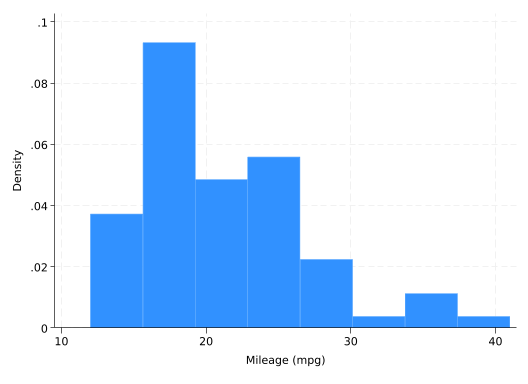
A histogram will tell you more about the distribution of a continuous variable than summary statistics, and they’re easy to make. Just run:
hist mpg
(bin=8, start=12, width=3.625)
There are several options to consider with histograms:
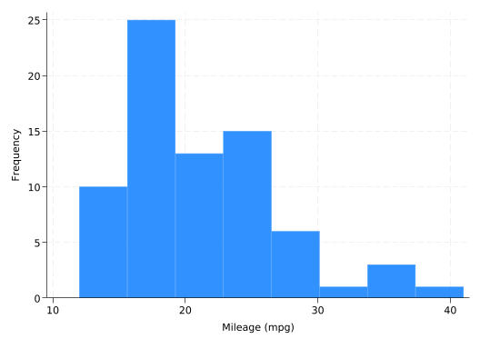
Stata likes to think of a histogram as an empirical approximation to a probability distribution function, but to get the kind of histogram you learned about in elementary school where the height of the bar is proportional to the number of observations in the bin, add the freq option:
hist mpg, freq
(bin=8, start=12, width=3.625)
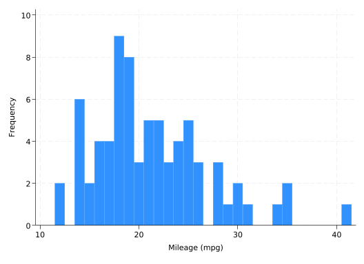
Use the bin() option to control the number of bins rather than letting Stata guess what would be appropriate:
hist mpg, freq bin(15)
(bin=15, start=12, width=1.9333333)
The discrete option tells Stata to make one bin for each value of the variable:
hist mpg, freq discrete
(start=12, width=1)
Choosing the number of bins can be something of an art: a histogram with too few bins can miss things, but so can a histogram with too many. Experiment a bit before settling on a number.
6.1.2 Categorical Variables
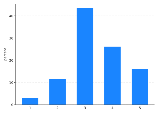
With categorical variables you’re interested in the frequencies. A bar graph won’t show you any more information than you’ll get by using tab to make a frequency table, but you can get a basic understanding of it in a single glance.
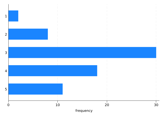
With the graph bar command you use the over() option to tell it the variable that defines the bars:
graphbar, over(rep78)
If you have labels for the bars (and you should) there’s a good chance the labels will overlap. This problem is goes away immediately if you use horizontal bars, made with graph hbar:
graphhbar, over(rep78)
By default, graph hbar (or graph bar) calculates the percentage of observations in each category. You can change that to frequencies by telling it you want to graph the (count):
graphhbar (count), over(rep78)
You can label the bars with those counts using the blabel(bar) option:
graphhbar (count), over(rep78) blabel(bar)
Now it really contains all the same information as a frequency table.
Bar graphs can get tricky. For more on how to create them and make them look presentable, see Bar Graphs in Stata.
6.2 Relationships Between Variables
Data visualizations are also a great tool for understanding the relationships between two or more variables.
6.2.1 One Continuous Variable and One Categorical Variable
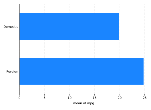
If you have a categorical variable and a continuous variable, one measure of the relationship between them is how the mean of the continuous variable varies across categories. graph hbar can do that with (mean) and then the name of the continuous variable:
graphhbar (mean) mpg, over(foreign)
This can tell you there’s a difference between the categories, but doesn’t tell you much about how the distribution of the continuous variable varies between them. A box plot will tell you more:
graph box mpg, over(foreign)
Working from the center out: the line in the middle of the box is the median, and the top and bottom of the box is the 75th and 25th percentile respectively. The “whiskers” outside the box go to the upper adjacent and lower adjacent values. (To find the upper/lower adjacent value, take the 75th/25th percentile, add/subtract 1.5 times the difference between the 75th and 25th percentile, and find the largest/smallest value below/above that number.) Observations outside of the whiskers get their own dot.
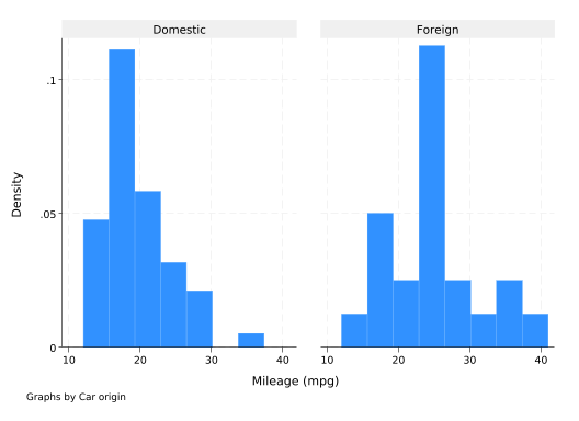
A simple alternative is to create a histogram for each category. You can do this by adding the by() option to the hist command. This is conceptually similar to the by prefix:
hist mpg, by(foreign)
6.2.2 Two Categorical Variables
Plotting relationships between two categorical variables can be fun, but it gets complicated. See Bar Graphs in Stata.
6.2.3 Two Continuous Variables
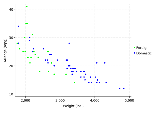
The classic plot for exploring the relationship between two continous variables is a scatterplot, easily created with scatter:
scatter mpg weight
6.2.4 Three Variables
You can add a third variable to the mix by having it determine the color of the points in a scatterplot. As of Stata 18, this can be done with the colorvar option. By default, Stata will treat the color variable as continuous:
scatter mpg weight, colorvar(displacement)
displacement is a measure of the size of a car’s engine. This plot shows us that there is a strong relationship between a car’s gas mileage, its weight, and the size of its engine.
It’s more common to use color to represent a categorical variable. You can tell Stata that the color variable is categorical with the colordiscrete option, but unfortunately you also have to tell it to use a sensible legend for categorical variables with coloruseplegend (don’t ask why it has that name) and to use the value labels in the legend with zlabel(, val).
This shows that foreign cars were generally smaller than domestic cars in 1978, but they frequently have lower gas mileage than domestic cars of comparable size.
6.3 Combining Plots
A scatterplot is an example of what Stata calls a twoway plot: a plot with a y and x axis. You can combine twoway plots by putting || (two pipe characters) between them. Each additional plot will go on top of the previous plots, like a coat of paint.
An lfit plot plots a linear fit (i.e. a univariate regression) of two variables. (There’s also qfit for quadratic fit, i.e. with a squared term.) Layer it over the scatterplot with:
scatter mpg weight || lfit mpg weight
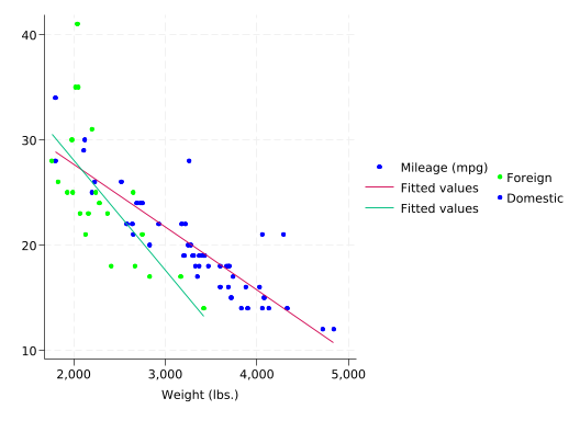
Now suppose you want foreign and domestic cars to be different colors in the scatterplot and we want two separate fit lines which are also different colors. You can get different colors in the scatterplot with colorvar(), but lfit doesn’t do colovar(). Instead, add two lfit plots, one for each subset of the data. This is a good time to use /// to continue a command on the next line:
This trick of getting different colors by using one plot for each subset of the data works any time colorvar() is not an option.
You’d obviously need to change the labels in the legend before you’d show this to anyone else, and that’s not something we’ll go into. But it’s perfectly adequate to help you understand the relationships between mpg, weight, and foreign.
6.4 Exporting Data Visualizations
To use a data visualization in something like a Word document or web page, you need to export it to an appropriate file format. We’ve found that .emf works well in Word, while .png works well for most other things. The graph export command will export the most recent graph to a file. It will determine the file format you want from the extension you use in the file name:
graphexport scatterplot.png, replace
file scatterplot.png written in PNG format
To wrap up your do file, add:
logclose
      name:  <unnamed>
       log:  /home/d/dimond/kb/stata_intro/data_viz.log
  log type:  text
 closed on:   4 Feb 2026, 15:56:29
-------------------------------------------------------------------------------