In this chapter we’ll discuss variable transformations: creating and changing variables. You should already be familiar with the basics of variable transformations–if you’re not, Introduction to Stata: Creating and Changing Variables will get you up to speed. This chapter will add to your “bag of tricks” for working with numeric data. You’ll learn some useful functions and commands, and generally gain experience writing Stata code.
4.1 Setting Up
Start a do file called numeric_transforms.do that loads acs.dta, either from the SSCC web site or locally if you downloaded the example files.
-------------------------------------------------------------------------------
      name:  <unnamed>
       log:  /home/d/dimond/kb/dws/transforms.log
  log type:  text
 opened on:  26 Nov 2025, 11:58:21
4.2 Transformations and Missing Data
If an observation has a missing value for a variable, it should usually, but not always, have a missing value for any transformations of that variable.
Arithmetic operators (addition, subtraction, etc.) do this automatically. For example, to correct the incomes in this year 2000 ACS data set for inflation, we can convert them to (January) 2025 dollars by multiplying them by 1.88. Look at the result for household 484:
gen income_2025 = income * 1.88list household person age income income_2025 if household==484, ab(30)
The two children in the household have missing values for income, so they automatically got a missing value for income_2025. This is almost always what you want.
However, egen functions behave differently. In general, they act on the observed data and ignore the missing data. For example, consider calculating household incomes using the egentotal function (and by):
by household: egen household_income = total(income)list household person age income household_income if household==484, ab(30)
The total function added up all the observed values of income and ignored the missing values. This had the effect of treating the missing values as zeros, but that isn’t a general rule. The mean function will calculate the mean of the observed values, which has the effect of treating missing values as if they were at the mean. Be sure to think through whether the behavior of egen makes sense for your particular task.
Conditions never return a missing value, even if they involve missing values. For example, consider creating an indicator for high_income with the threshold for “high” being $50,000:
gen high_income_oops = (income > 50000)list household person age income high_income_oops if household==484, ab(30)
Recall that the way Stata handles missing values is to designate the 27 largest possible values of each variable type as the various flavors of missing (., .a, .b, .c, up though .z). But when it comes to conditions (unlike arithmatic operators or egen functions) missing values are just treated like the big numbers they really are. Thus the following inequalities hold:
Missing Values and Inequalities
Any observed value or normal number < . < .a < .b < .c … < .x < .y < .z
That’s why the children, with their missing values for income, got a 1 for high_income: to Stata . is biggger than 50000 or any other number.
The solution is to exclude observations with missing values from the process of creating the new variable entirely. Thus they’ll be left with a missing value, which is what you want.
gen high_income= (income > 50000) if income < .list household person age income high_income if household==484, ab(30)
Why income < . rather than income != .? Because income < . excludes all the missing values (., .a, .b, etc.), not just ..
However, subtle differences in what you want your variable to mean can change how you handle missing values. Suppose you wanted an indicator for “this person is known to have a high income.” Now anyone with a missing value for income should have a 0 for the new indicator because they are not known to have a high income. But you can’t just ignore the missing values, or people with a missing value will get a 1. Instead, a person should get a 1 for known_high_income if their income is both high and known:
gen known_high_income = (income > 50000) & (income < .)list household person age income known_high_income if household==484, ab(30)
Create an indicator variable married_woman which should get a 1 of for people who are married and female (regardless of age), a 0 for people who are not married and female, and a missing value for people where we can’t tell which value they should get. You’ll need to remind yourself which value of marital_status means married. Recall that while the Census Bureau assumed that children under the age of 15 could not be married, in the last chapter we decided to treat their marital status as unknown (since the Census Bureau didn’t ask) and changed their value of marital_status to missing.
Solution
First, a look at marital_status. You can identify which values go with which labels by running first tab and then tab with the nolabel option:
tab marital_status, missing
      Marital |
       Status |      Freq.     Percent        Cum.
--------------+-----------------------------------
  Now married |     11,643       42.48       42.48
      Widowed |      1,405        5.13       47.60
     Divorced |      2,177        7.94       55.55
    Separated |        435        1.59       57.13
Never married |      5,606       20.45       77.58
            . |      6,144       22.42      100.00
--------------+-----------------------------------
        Total |     27,410      100.00
As usual, you need to think through the missing values. A male cannot be a married woman regardless of his marital status, even if it’s missing, so you can’t use just if marital_status<. to set the new variable to missing if marital_status is missing.
gen married_woman = female & marital_status==1 if !female | marital_status<.
(2,998 missing values generated)
If someone has a missing value for marital_status, then female & marital_status==1 will be false (0) because the second condition is false. If they are male (!female) then that result is correct and we want to use it. Only if they’re female should we require that marital_status be non-missing in order to use the result.
4.3 Conditional Transformations (Transformations that Vary for Subsets)
Often a variable transformation must be different for different subsets of the data. As a trivial example, suppose you wanted to define an education score for each person which is:
25 if they do not have a bachelor’s degree
75 if they do have a bachelor’s degree or higher
We’ll explore several ways of creating this ed_score variable.
First off, let’s remind ourselves how edu is defined so we can figure out how to identify people with bachelor’s degrees or higher. Run describe edu to get the name of the value labels associated with it:
describe edu
Variable      Storage   Display    Value
    name         type    format    label      Variable label
-------------------------------------------------------------------------------
edu             byte    %24.0g     edu_label
                                              Educational Attainment
Next use label list edu_label to see what the labels mean:
labellist edu_label
edu_label:
           0 Not in universe
           1 None
           2 Nursery school-4th grade
           3 5th-6th grade
           4 7th-8th grade
           5 9th grade
           6 10th grade
           7 11th grade
           8 12th grade, no diploma
           9 High School graduate
          10 Some college, <1 year
          11 Some college, >=1 year
          12 Associate degree
          13 Bachelor's degree
          14 Master's degree
          15 Professional degree
          16 Doctorate degree
The presence of the “Not in universe” label is a good reminder that the Census Bureau did not collect education data for people under the age of three, so we set those values to missing. But let’s assume that no one under the age of three can possibly have a bachelor’s degree.
The values 13, 14, 15, and 16 indicate a bachelor’s degree or higher, or, to put it more succinctly, edu>=13. Remember that Stata considers missing to be greater than 13, but people with a missing value of edu are under the age of three and we assume that no one under the age of three has a bachelor’s degree. Thus the complete condition for identifying people with a bachelor’s degree is (edu >= 13) & (edu < .).
Since we’ll need to identify people with a bachelor’s degree condition multiple times, it will be convenient to create an indicator variable for it so we don’t have to type out the full condition every time:
gen bachelors = (edu >= 13) & (edu < .)
The straightforward way to create ed_score is two commands that essentially translate the original definition into Stata:
gen ed_score = 25 if !bachelorsreplace ed_score = 75 if bachelorslist household person edu ed_score in 1/5, ab(30)
(4,485 missing values generated)
(4,485 real changes made)

     +--------------------------------------------------------+
     | household   person                      edu   ed_score |
     |--------------------------------------------------------|
  1. |        37        1   Some college, >=1 year         25 |
  2. |        37        2   Some college, >=1 year         25 |
  3. |        37        3   Some college, >=1 year         25 |
  4. |       241        1          Master's degree         75 |
  5. |       242        1        Bachelor's degree         75 |
     +--------------------------------------------------------+
That works just fine for this simple example. But if this were just part of a more complex calculation it would be useful to have a single mathematical expression that can calculate both values. You can do that using the cond() function. The cond() function takes three arguments:
A condition
The result if the condition is true
The result if the condition is false
In this case, the first argument could be either (edu >= 13) & (edu < .) or just the indicator variable bachelors. If that is true, then the person has a bachelor’s degree or higher and the education score should be 75, so 75 is the second argument. If that is false, the person does not have a bachelor’s degree and education score should be 25, so 25 is the third argument.
gen ed_score2 = cond(bachelors, 75, 25)list household person edu ed_score2 in 1/5, ab(30)
     +---------------------------------------------------------+
     | household   person                      edu   ed_score2 |
     |---------------------------------------------------------|
  1. |        37        1   Some college, >=1 year          25 |
  2. |        37        2   Some college, >=1 year          25 |
  3. |        37        3   Some college, >=1 year          25 |
  4. |       241        1          Master's degree          75 |
  5. |       242        1        Bachelor's degree          75 |
     +---------------------------------------------------------+
An alternative way of looking at this notes that you can think of the original definition of education score as saying that everyone starts with an education score of 25 points, and then people with a bachelor’s degree or higher get an additional 50 points. That can be implemented with:
gen ed_score3 = 25replace ed_score3 = ed_score3 + 50 if bachelorslist household person edu ed_score3 in 1/5, ab(30)
(4,485 real changes made)

     +---------------------------------------------------------+
     | household   person                      edu   ed_score3 |
     |---------------------------------------------------------|
  1. |        37        1   Some college, >=1 year          25 |
  2. |        37        2   Some college, >=1 year          25 |
  3. |        37        3   Some college, >=1 year          25 |
  4. |       241        1          Master's degree          75 |
  5. |       242        1        Bachelor's degree          75 |
     +---------------------------------------------------------+
Setting a variable equal to itself plus something is a very common and useful pattern.
Now consider this alternative:
gen ed_score4 = 25 + 50*bachelorslist household person edu ed_score4 in 1/5, ab(30)
     +---------------------------------------------------------+
     | household   person                      edu   ed_score4 |
     |---------------------------------------------------------|
  1. |        37        1   Some college, >=1 year          25 |
  2. |        37        2   Some college, >=1 year          25 |
  3. |        37        3   Some college, >=1 year          25 |
  4. |       241        1          Master's degree          75 |
  5. |       242        1        Bachelor's degree          75 |
     +---------------------------------------------------------+
bachelors is either 1 or 0. For people without a bachelor’s degree it is 0, so 50 multiplied by 0 goes away and they just get the original 25. For people with a bachelor’s degree it is 1, so 50 is multiplied by 1 and they get a total of 75.
This is exactly how indicator variables work in regression models. If this were a regression model, 25 would be the constant, 50 would be the coefficient on the indicator covariate bachelors, and the predicted value would be either 25 or 75.
Interaction terms are very similar. If 50 were the coefficient on an interaction between bachelors and age, then it would be 50 * bachelors * age. Again the entire term disappears (is multiplied by 0) for people who do not have a bachelor’s degree, and it becomes just 50*age for people who do.
All of these could be done using the original condition (edu>=13) & (edu<.) rather than the indicator bachelors, even the last version.
gen ed_score5 = 25 + 50*((edu>=13) & (edu<.))list household person edu ed_score5 in 1/5
     +-------------------------------------------------------+
     | househ~d   person                      edu   ed_sco~5 |
     |-------------------------------------------------------|
  1. |       37        1   Some college, >=1 year         25 |
  2. |       37        2   Some college, >=1 year         25 |
  3. |       37        3   Some college, >=1 year         25 |
  4. |      241        1          Master's degree         75 |
  5. |      242        1        Bachelor's degree         75 |
     +-------------------------------------------------------+
When a condition appears in a mathematical expression, Stata automatically recognizes it, the result is either 0 or 1, and that is used in evaluating the rest.
4.4 Conditions with Many Values
The values of edu that mean “bachelor’s degree or higher” are 13, 14, 15, and 16. It’s highly convenient to specify them using the inequalities (edu >= 13) & (edu < .) and by all means you should do that where possible. But sometimes the values you need don’t match a simple pattern and you need to list them all. You could specify them with a series of conditions combined with logical or:
(edu==13) | (edu==14) | (edu==15) | (edu==16)
You’re probably thinking “Surely there’s an easier way” and there is: the inlist() function. The first argument of inlist() is a variable, and the rest are possible values of that variable. The result is 1 (true) if the actual value of the variable is in the list, and 0 (false) if it is not. Use it wherever you would use a condition, including inside mathematical expressions:
gen bachelors2 = inlist(edu, 13, 14, 15, 16)gen ed_score6 = 25 + 50*inlist(edu, 13, 14, 15, 16)list household person edu bachelors2 ed_score6 in 1/5, ab(30)
     +----------------------------------------------------------------------+
     | household   person                      edu   bachelors2   ed_score6 |
     |----------------------------------------------------------------------|
  1. |        37        1   Some college, >=1 year            0          25 |
  2. |        37        2   Some college, >=1 year            0          25 |
  3. |        37        3   Some college, >=1 year            0          25 |
  4. |       241        1          Master's degree            1          75 |
  5. |       242        1        Bachelor's degree            1          75 |
     +----------------------------------------------------------------------+
Note that you can also use inlist() with a string variable, in which case the values must be strings.
The related inrange() function takes three arguments: a variable, and the beginning and end of a range. It returns 1 if the variable is in the range specified and 0 otherwise.
gen bachelors3 = inrange(edu, 13, 16)list household person edu bachelors3 in 1/5, ab(30)
     +----------------------------------------------------------+
     | household   person                      edu   bachelors3 |
     |----------------------------------------------------------|
  1. |        37        1   Some college, >=1 year            0 |
  2. |        37        2   Some college, >=1 year            0 |
  3. |        37        3   Some college, >=1 year            0 |
  4. |       241        1          Master's degree            1 |
  5. |       242        1        Bachelor's degree            1 |
     +----------------------------------------------------------+
Exercise
Given the automobile dataset that comes with Stata, suppose the price of manufacturing a car is to total of:
$1.50 per pound of weight
$0.25 per pound to ship if it is foreign
$100 if its rep78 is 4 or 5
A student tries to calculate the total cost of manufacturing a car with the following code:
clearsysuse autogen base_cost = 1.5*weightgen shipping_cost = .25*weightif foreigngen quality_cost = 100 if rep78==4 | rep78==5gen total_cost = base_cost + shipping_cost + quality_costlist make total_cost in 1/3
Why doesn’t this work? Carry out the task correctly.
Reload the ACS when you’re done.
Solution
The trouble lies with how the student calculated shipping_cost and quality_cost. shipping_cost is not zero for domestic cars, it is missing. Similarly, quality_cost is missing for cars that do not have a 4 or 5 for rep78. Thus adding them up gives mostly missing values.
There are several ways to do this properly. The following code is simple and easy to understand:
gen cost1 = 1.5*weightreplace cost1 = cost1 + .25*weightif foreignreplace cost1 = cost1 + 100 if rep78==4 | rep78==5
(22 real changes made)
(29 real changes made)
The following code is more concise:
gen cost2 = 1.5*weight + .25*weight*foreign + 100*inlist(rep78, 4, 5)
Early in your Stata career you might be better off using the first version, and move to the second only when it starts becoming intuitive to you.
Neither version deals with missing values. If rep78 is unknown, then cost is unknown, but this will not happen automatically with either method. So do it explicitly:
replace cost1 = . if rep78==.replace cost2 = . if rep78==.
(5 real changes made, 5 to missing)
(5 real changes made, 5 to missing)
Dividing a data set into quantiles is a very common task, and is easily carried out using the xtile command. For example, you can assign the adults in the ACS to their income quintile with:
xtile inc_quint = income if age>=18, n(5)
The n() option specifies the number of quantiles.
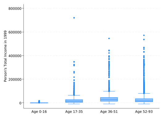
The result will be an ordered categorical variable, frequently used for grouping with the by prefix or with over() in graphs. For example, you can create a box plot of income over the five quintiles with:
graph box income, over(inc_quint)
Exercise
Create a variable containing quartiles for age, then make a box plot of income over the age quartiles. Apply value labels to the quartiles that specify the age range they cover.
Solution
xtile age_quartile = age, n(4)
To set the value labels, you need to know the minimum and maximum age in each quartile.
bysort age_quartile: sum age
-------------------------------------------------------------------------------
-> age_quartile = 1

    Variable |        Obs        Mean    Std. dev.       Min        Max
-------------+---------------------------------------------------------
         age |      6,932    8.183785    4.837898          0         16

-------------------------------------------------------------------------------
-> age_quartile = 2

    Variable |        Obs        Mean    Std. dev.       Min        Max
-------------+---------------------------------------------------------
         age |      6,988    26.32885    5.488741         17         35

-------------------------------------------------------------------------------
-> age_quartile = 3

    Variable |        Obs        Mean    Std. dev.       Min        Max
-------------+---------------------------------------------------------
         age |      6,700     43.1594    4.547501         36         51

-------------------------------------------------------------------------------
-> age_quartile = 4

    Variable |        Obs        Mean    Std. dev.       Min        Max
-------------+---------------------------------------------------------
         age |      6,790    65.97202    10.28828         52         93
Note that running bysort age_quartile changed the order of the data. You’re used to the first five observations being all the members from households 37, 241, and 242, but now they’re children from random households. Put the data back in the original order before proceeding.
sort household person
4.6 Creating Categorical Variables From Cutpoints
An alternative way to use xtile is to define a categorical variable based on a continuous variable with cutpoints that define the categories. As an example, we’ll use it to categorize age by decade (20s, 30s, etc.).
The cutpoints must be put in a variable in the data set, normally one you’ll create just for this purpose. But the values won’t actually belong to the observations they’re attached to. Rather the value of the cutpoint for the first observation will be the maximum value for the first category, the value for the second observation will be the maximum for the second category, etc. The maximum value is included in the category (i.e. the rule is value <= max). You should have more observations than categories, so the rest will get missing values. Normally you’ll drop this variable as soon as you’re done with it.
For decades we want the cutpoints to be 9, 19, 29 up through 99 (recall that in the ACS 93 really means “93 or older”). You can do that with:
gen cutpoints = _n*10 - 1 if_n<=10list cutpoint in 1/12, ab(30)
Technically, we don’t need the last cutpoint (99). There’s always an implied additional category for “everything greater then the final cutpoint.” We could have just stopped at 89 and let Stata put everything above that in the final category automatically, but given how we defined the cutpoints it wasn’t any more work to put in 99.
Having defined your cutpoints, you can now run xtile with the cut() option, which tells it to use cutpoints instead of quantiles and gives the name of the variable that contains the cutpoints.
xtile decade = age, cut(cutpoints)list household person age decade in 1/5
The categories seem off because they are numbered starting with 1, so right now a 1 for decade means ages 0-9, 2 means ages 10-19, etc. While the values of a categorical variable are completely arbitrary in theory, if you subtract 1 and then multiply by 10, 0-9 will be 0, 10-19 will be 10, 20-29 will be 20, etc. and that’s a good bit more intuitive.
replace decade = (decade - 1)*10list household person age decade in 1/5
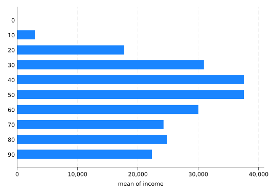
Now it’s ready for use, for example, plotting the mean income by decade:
graphhbar income, over(decade)
You can easily set completely arbitrary cutpoints using the input command. You give the command, the name of a variable to be created, and then one value of the variable per line, stopping with end:
input age_cats 19 30endxtile age_cat = age, cut(age_cats)list household person age age_cats age_cat in 1/5
To demonstrate that the categories are defined correctly:
bysort inc_cat: sum income
-------------------------------------------------------------------------------
-> inc_cat = 1

    Variable |        Obs        Mean    Std. dev.       Min        Max
-------------+---------------------------------------------------------
      income |      2,608   -36.73696    490.9712     -10000          0

-------------------------------------------------------------------------------
-> inc_cat = 2

    Variable |        Obs        Mean    Std. dev.       Min        Max
-------------+---------------------------------------------------------
      income |      8,841    9769.877    5769.632          4      20000

-------------------------------------------------------------------------------
-> inc_cat = 3

    Variable |        Obs        Mean    Std. dev.       Min        Max
-------------+---------------------------------------------------------
      income |      6,930    32814.16    8317.071      20004      50000

-------------------------------------------------------------------------------
-> inc_cat = 4

    Variable |        Obs        Mean    Std. dev.       Min        Max
-------------+---------------------------------------------------------
      income |      2,180    67219.41    13439.32      50004     100000

-------------------------------------------------------------------------------
-> inc_cat = 5

    Variable |        Obs        Mean    Std. dev.       Min        Max
-------------+---------------------------------------------------------
      income |        707    182971.3    91980.77     100020     720000

-------------------------------------------------------------------------------
-> inc_cat = .

    Variable |        Obs        Mean    Std. dev.       Min        Max
-------------+---------------------------------------------------------
      income |          0
But put the data back in order:
sort household person
4.7 Extracting Digits From Numbers
You may be thinking “That’s nice, but couldn’t we have gotten decade by just dividing age by 10?” Almost: you want to divide by ten and get rid of the fractional part. You can do that by telling Stata that the new variable you’re creating should be an integer:
genint decade2 = age/10list household person age decade2 in 1/5
Stata will do the division normally but, because the decade2 variable is an integer, when it comes time to store the result any fractional part is discarded. Thus if age/10 is 1.9, only the 1 is stored. This integer division is surprisingly useful.
Note that this time ages 0-9 are decade 0, but you probably still want to multiply by 10 so 20-29 is 20 instead of 2.
replace decade2 = decade2 * 10list household person age decade in 1/5
If you wanted just the last digit of age, you could get that with the mod() (modulus) function. It takes two arguments and returns the remainder when the first is divided by the second:
genyear = mod(age, 10)list household person age yearin 1/5
The combination of integer division and modulus allows you to split up numbers at will. For example, the FIPS code for Dane County, Wisconsin is 55025, where 55 is the code for Wisconsin. But if you want to do analysis at the state and county level, you may need separate state and county variables. You can do that with:
gen fips = 55025genint state = fips/1000gen county = mod(fips, 1000)list fips state county in 1
     +------------------------+
     |  fips   state   county |
     |------------------------|
  1. | 55025      55       25 |
     +------------------------+
(Note that for many purposes you can use state plus the original FIPS code, as the original FIPS code uniquely identifies counties.)
The county variable does not include a leading zero–numeric variables never do. Most of the time that’s not a problem: FIPS codes do not use 25 and 025 to mean different counties. You can tell Stata to print a numeric variable with leading zeros. But if you really need 25 and 025 to mean different things store the variable as a string.
Exercise
Create a variable containing the telephone number 6082629917. Extract the area code. Then extract the last four digits.
Hint: When you think of 6082629917 as a single number rather than a series of digits, it’s a really big number–too big to store in the default float variable type without it being rounded.
Solution
Phone numbers with area codes must be stored as double precision numbers (or strings, if you don’t need to do any math with them). Try leaving out double in the following code to see why.
You might be tempted to think of the integer division like gen int decade2 = age/10 as “rounding to the nearest 10”, but it’s actually quite different from rounding. You’ll see why if you generate decade3 by actually rounding to the nearest 10. The round() function takes two arguments: the number to be rounded, and the number to round to.
gen decade3 = round(age, 10)list household person age decade2 decade3 in 1/5