4  First Steps With Your Data

Once you’ve read in a new data set, your first goals are to understand the data set and to clean it up. Logically these are two separate processes, but in practice they are intertwined: you can’t clean your data set until you understand it at some level, but you won’t fully understand it until it’s clean. Thus this section will cover both.

We’ll also introduce a lot of data science concepts in this section. This makes for lengthy discussions of tasks that in practice you can complete very quickly.

In this chapter we’ll primarily use the file 2000_acs_sample.csv. This file started as the 1% unweighted sample of the 2000 American Community Survey available from IPUMS, but then I took a 1% random sample of the households in that data set just to make it easier to work with. This data set uses the ‘source’ variables directly from the Census Bureau rather than the ‘harmonized’ variables created by IPUMS, which are much cleaner. For real work you can usually use the harmonized variables, but we’re here to learn how to do the kinds of things IPUMS does to create them. We use the 2000 ACS because it’s the last one to be unweighted, and we don’t want to deal with weights right now.

By using this data set in the examples you’ll gain some basic understanding of the U.S. population (as of 2000 anyway) and some experience with a real and important data set, but you would not want to use this particular data file for research.

4.1 Setting Up

Start up Jupyter Lab if you haven’t already and navigate to the folder where you put the example files. Then create a new Python Notebook and call it First_Steps_Practice.ipynb. Have it import Pandas and then use the Pandas read_csv() function to read in 2000_acs_sample.csv:

import pandas as pd
acs = pd.read_csv('2000_acs_sample.csv')

4.2 Read the Documentation

When you download a data set, you’ll be tempted to open it up and go to work right away. Resist! Time spent reading the data set’s documentation (assuming there is any) can save you much more time down the road. Data providers may give you files containing documentation along with the data itself, or it may be on their web site. Feel free to skim what’s not relevant to you–this chapter will give you a better sense of what information is most important.

Unfortunately, not all data sets have good documentation, or any documentation at all, so figuring out the nature of a data set by looking at the data set itself is a vital skill. You also can’t assume that the documentation is completely accurate, so you need to check what it says.

The ACS has lots of good documentation, but for practice we’ll make minimal use of it (just the codebook) and figure out everything we can for ourselves. We’d still do all the same things if we were using the documentation, we’d just understand what we were looking at much more quickly.

4.3 Identify the Variables

To see what variables the data set contains, look at its dtypes (data types):

acs.dtypes

year                 int64
datanum              int64
serial               int64
hhwt                 int64
gq                  object
us2000c_serialno     int64
pernum               int64
perwt                int64
us2000c_pnum         int64
us2000c_sex          int64
us2000c_age          int64
us2000c_hispan       int64
us2000c_race1        int64
us2000c_marstat      int64
us2000c_educ         int64
us2000c_inctot      object
dtype: object

The primary goal of looking at the dtypes is to see what variables you have and what they’re called. But it will frequently let you start a “to do list” of issues you need to address before analyzing the data. Here are some issues brought out by running describe on this data set:

1. The data set seems to have an excess of identifiers: serial, us2000c_serialno, pernum and us2000c_pnum

2. Since you’re using a single data set from a single year, you don’t need year and datanum to tell you where each observation come from.

3. For the same reason, you also don’t need us2000c_ (‘US 2000 Census’) in your variable names to tell you where those variables come from.

4. You have both household weight (hhwt) and person weight (pwt) variables even though this is supposed to be an unweighted sample.

5. us2000c_inctot is stored as an object, probably a string, even though it should presumably be numeric. (We’ll have to investigate gq.)

Exercise

Read in 2000_acs_harm.csv as acs_harm and examine its dtypes. This is a similar sample but with the IPUMS ‘harmonized’ variables. What issues did IPUMS resolve? What issues remain?

Solution

acs_harm = pd.read_csv('2000_acs_harm.csv')
acs_harm.dtypes

year        int64
datanum     int64
serial      int64
hhwt        int64
gq         object
pernum      int64
perwt       int64
sex        object
age        object
marst      object
race       object
raced      object
hispan     object
hispand    object
educ       object
educd      object
inctot      int64
ftotinc     int64
dtype: object

• The excess identifiers are gone
• The unneeded year and datanum variables are still there
• The US200c_ prefixes are gone
• The weights are still there
• inctot and ftotinc are numeric, but gq is still an object.
• We seem to have picked up d versions of some variables (raced, hispand, educd)

4.4 Look at the Data

Unless your data set is very small, you can’t possibly read all of it. But just looking at what JupyterLab’s implicit print will give you may allow you to immediately spot patterns that would be difficult to detect using code:

acs

	year	datanum	serial	hhwt	gq	us2000c_serialno	pernum	perwt	us2000c_pnum	us2000c_sex	us2000c_age	us2000c_hispan	us2000c_race1	us2000c_marstat	us2000c_educ	us2000c_inctot
0	2000	4	37	100	Households under 1970 definition	365663	1	100	1	2	20	1	1	5	11	0010000
1	2000	4	37	100	Households under 1970 definition	365663	2	100	2	2	19	1	1	5	11	0005300
2	2000	4	37	100	Households under 1970 definition	365663	3	100	3	2	19	1	2	5	11	0004700
3	2000	4	241	100	Households under 1970 definition	2894822	1	100	1	2	50	1	1	5	14	0032500
4	2000	4	242	100	Households under 1970 definition	2896802	1	100	1	2	29	1	1	5	13	0030000
...	...	...	...	...	...	...	...	...	...	...	...	...	...	...	...	...
28167	2000	4	1236624	100	Households under 1970 definition	7055193	1	100	1	1	29	1	1	1	11	0050100
28168	2000	4	1236624	100	Households under 1970 definition	7055193	2	100	2	2	26	1	1	1	9	0012000
28169	2000	4	1236756	100	Households under 1970 definition	8489120	1	100	1	2	58	1	1	1	14	0069800
28170	2000	4	1236756	100	Households under 1970 definition	8489120	2	100	2	1	61	1	1	1	14	0040800
28171	2000	4	1236779	100	Households under 1970 definition	8733299	1	100	1	1	30	1	3	3	9	0022110

28172 rows × 16 columns

Some things to notice:

• year and datanum seem to have just one value each, suggesting that we don’t need them.

• hhwt and perwt (household and person weights) seem to always be 100, which makes sense given that this is supposed to be an unweighted sample.

• pernum and us2000c_pnum appear to be identical.

• pernum seems to count observations, starting over from 1 every time serial changes.

• us2000c_sex, us2000c_hispan, us2000c_race1, and us2000c_marstat are clearly describing categories. We will have to refer to the codebook to find out what the numbers mean. (This also applies to us2000c_educ, it’s just not as obvious at this point.)

You can’t be sure that these patterns hold the for entire data set until you check using methods that examine the entire data set. The value_counts() function will give you frequencies for a variable:

acs['year'].value_counts()

year
2000    28172
Name: count, dtype: int64

There is indeed just one value of year, 2000, the year the data were collected. This might be useful if we were combining data sets from different years, but since we’re not you’ll soon learn how to drop it.

Exercise

Use value_counts() to get the frequencies of datanum, hhwt, and perwt.

Solution

Remember you only get one implicit print per cell, so unless you want to use three cells use the print() function.

print(acs['datanum'].value_counts())
print(acs['hhwt'].value_counts())
print(acs['perwt'].value_counts())

datanum
4    28172
Name: count, dtype: int64
hhwt
100    28172
Name: count, dtype: int64
perwt
100    28172
Name: count, dtype: int64

Or if you’re feeling lazy (in public we call it being efficient):

for var in ['datanum', 'hhwt', 'perwt']:
    print(acs[var].value_counts())

datanum
4    28172
Name: count, dtype: int64
hhwt
100    28172
Name: count, dtype: int64
perwt
100    28172
Name: count, dtype: int64

Either way, all three variables have just one value throughout the entire data set and thus convey no information. We’ll drop them soon.

Exercise

Examine acs_harm in the same way. What issues do you see? Be sure to take a close look at inc_tot.

Solution

acs_harm

	year	datanum	serial	hhwt	gq	pernum	perwt	sex	age	marst	race	raced	hispan	hispand	educ	educd	inctot	ftotinc
0	2000	4	202721	100	Households under 1970 definition	3	100	Female	7	Never married/single	White	White	Not Hispanic	Not Hispanic	Nursery school to grade 4	Nursery school to grade 4	9999999	100000
1	2000	4	1204668	100	Households under 1970 definition	7	100	Male	11	Never married/single	Black/African American/Negro	Black/African American/Negro	Not Hispanic	Not Hispanic	Grade 5, 6, 7, or 8	Grade 5 or 6	9999999	52700
2	2000	4	78909	100	Households under 1970 definition	3	100	Male	16	Never married/single	Two major races	White and other race write_in	Other	Other, n.s.	Grade 10	Grade 10	15000	74900
3	2000	4	570434	100	Households under 1970 definition	1	100	Male	32	Married, spouse present	White	White	Other	Guatemalan	Grade 12	12th grade, no diploma	18000	18000
4	2000	4	620890	100	Households under 1970 definition	1	100	Male	52	Married, spouse present	White	White	Not Hispanic	Not Hispanic	4 years of college	Bachelor's degree	59130	100800
...	...	...	...	...	...	...	...	...	...	...	...	...	...	...	...	...	...	...
28080	2000	4	647711	100	Households under 1970 definition	2	100	Male	50	Separated	Black/African American/Negro	Black/African American/Negro	Not Hispanic	Not Hispanic	Grade 5, 6, 7, or 8	Grade 5 or 6	16000	27400
28081	2000	4	512366	100	Households under 1970 definition	1	100	Male	38	Married, spouse present	Chinese	Chinese	Not Hispanic	Not Hispanic	5+ years of college	Professional degree beyond a bachelor's degree	48000	48000
28082	2000	4	155904	100	Other group quarters	1	100	Female	21	Never married/single	Black/African American/Negro	Black/African American/Negro	Not Hispanic	Not Hispanic	1 year of college	1 or more years of college credit, no degree	820	9999999
28083	2000	4	365991	100	Households under 1970 definition	4	100	Male	7	Never married/single	White	White	Not Hispanic	Not Hispanic	Nursery school to grade 4	Nursery school to grade 4	9999999	35800
28084	2000	4	614032	100	Households under 1970 definition	3	100	Female	15	Never married/single	White	White	Not Hispanic	Not Hispanic	Grade 5, 6, 7, or 8	Grade 7 or 8	0	41600

28085 rows × 18 columns

What most stands out is how variables like race and marital_status are now text rather than numbers, which makes them much more useful. More on that later. Now how some variables still do not appear to vary.

But looking at inctot we have some remarkably high incomes: $9,999,999. Oddly, we have multiple people with the exact same number. But what makes that really striking is that they’re all young children. In reality, 9999999 is a code for missing, and if you don’t fix that it will cause major problems for your analysis. We’ll learn how soon.

4.5 Identify the Indexes and Investigate the Structure of the Data

Logically, row indexes should uniquely identify a row. (Python does not actually enforce this, but duplicate indexes can cause performance problems. More importantly, they don’t make sense.) Back in the DataFrames chapter, we used person as the row index in the small extract from this data set that we examined. In this not-yet-cleaned-up data set it’s called pernum, but it clearly does not uniquely identify rows. That’s an important clue about the structure of the data: there’s more going on here than just people.

Suppose that I gave you some ‘student data’ and you found that student_id uniquely identified the rows. Then you could reasonably conclude that each row represents a student.

But suppose you found instead that each value of student_id was associated with multiple rows, but a combination of student_id and class_id uniquely identified the rows. That would tell you that each row represents a student-class combination, or a class taken by a particular student. We might just call each row a class, as long as it’s understood that two students taking the same class will be two rows.

This is critical information, and if you come to the SSCC’s statistical consultants for help you’re likely to be asked what a row represents in your data set. You might be surprised by how often the answer we get turns out to be wrong. (“What does a row represent in your data set?” “A patient.” “Then why do these five rows all have the same patient_id?” “They’re different doctor visits.” “Ah, then a row represents a doctor visit in your data set.”) Ideally the data documentation will tell you what the structure of the data set is, but it’s easy to check and well worth doing.

One way to easily check if pernum is a unique identifier is to look at its frequencies with value_counts():

acs['pernum'].value_counts()

pernum
1     11327
2      7786
3      4374
4      2689
5      1210
6       450
7       177
8        81
9        34
10       21
11       11
12        8
13        1
14        1
15        1
16        1
Name: count, dtype: int64

Note that the result is a Series, with the values of pernum as the index and the corresponding frequencies as values.

There are over 11,000 person 1’s, so clearly pernum is not a unique identifier. How about serial?

acs['serial'].value_counts()

serial
1115231    16
562736     12
962652     12
1122678    12
1110995    12
           ..
790922      1
227103      1
227189      1
790501      1
1236779     1
Name: count, Length: 11327, dtype: int64

We can’t see all the values of serial, but one of them is associated with 16 rows so once again we know it is not a unique identifier.

How about the combination of serial and pernum? If we give value_counts() two columns to act on, it will tell us the frequency of each combination of them (i.e. a crosstab). So select both columns by subsetting with a list:

acs[['serial', 'pernum']].value_counts()

serial   pernum
37       1         1
829137   2         1
830078   2         1
         1         1
829441   1         1
                  ..
428384   1         1
428351   8         1
         7         1
         6         1
1236779  1         1
Name: count, Length: 28172, dtype: int64

All the combinations we can see have just one row, but that’s a tiny fraction of the data set. How can we be sure?

The max() function finds the maximum value of a Series, like the Series of frequencies created by value_counts(). Try it first on the frequencies of serial:

acs['serial'].value_counts().max()

16

Since that gave us 16 as expected, now try it with the combination of serial and pernum:

acs[['serial', 'pernum']].value_counts().max()

1

With a maximum frequency of one, we now know that the combination of serial and pernum uniquely identifies the rows within this data set. In fact serial is a household identifier and pernum identifies a person within that household. We now know that this data set consists of people who are grouped into households.

When a combination of two or more variables uniquely identifies observations this is often known as a compound identifier, but Python calls it a MultiIndex. MultiIndex is actually a class in the Pandas package, though we’ll normally only use it in the context of a DataFrame.

It would make sense to set serial and pernum as the row indexes now, but we want to rename them first and we don’t yet know how to do that. So hold that thought.

Exercise

Read in the data set atus.csv as atus. This is a selection from the American Time Use Survey, which measures how much time people spend on various activities. Find the identifiers in this data set. What does an observation represent? What was the first activity recorded for person 20170101170012?

Solution

atus = pd.read_csv('atus.csv')
atus.dtypes

year           int64
caseid         int64
famincome     object
pernum         int64
lineno         int64
wt06         float64
age            int64
sex           object
race          object
hispan        object
asian         object
marst         object
educ          object
educyrs       object
empstat       object
fullpart      object
uhrsworkt      int64
earnweek     float64
actline        int64
activity      object
duration       int64
dtype: object

caseid, pernum, lineno, actline and activity stand out as possible identifiers. (Remember, identifiers generally don’t contain data.) None of them are unique identifiers alone, so you need to look for a combination that unique identifies the observations. For example:

atus[['caseid', 'pernum']].value_counts().max()

90

This pair does not uniquely identify all the observations (in fact, if you take off the max() you’ll see it doesn’t uniquely identify any). The correct pair turns out to be:

atus[['caseid', 'actline']].value_counts().max()

1

This tells us we have one observation per case (person) per activity. (activity turns out to be a label for the activity, not an identifier.) To see the first activity for person 20170101170012, use:

atus.loc[(atus['caseid']==20170101170012) & (atus['actline']==1), 'activity']

19    Sleeping
Name: activity, dtype: object

The ATUS starts tracking activities at 4:00AM, so for most people the first activity is sleeping.

4.6 Get Rid of Data You Won’t Use

Understanding data takes time. Even skipping past data you don’t care about to get to what you do care about takes time. So if you won’t use parts of a data set, get rid of those parts sooner rather than later. Doing so will also reduce the amount of memory needed to analyze your data and the amount of disk space needed to store it, and make anything you do with it run that much faster. If you change your mind about what you need, you can always change your code and rerun it later.

You can drop variables from a dataset with the DataFrame function drop(). You’ll need to pass in a variable name or list of names, plus axis=1 to tell it you want to drop columns rather than rows. .

We’ve determined that year, datanum, hhwt, and perwt contain no useful information (to us). Also, us2000c_pnum is identical to pernum, and us2000c_serialno appears to be an alternative version of serial that we don’t need. Remove them with:

acs = acs.drop(
    [
        'year',
        'datanum',
        'hhwt',
        'perwt',
        'us2000c_pnum',
        'us2000c_serialno'
    ],
    axis=1
)
acs

	serial	gq	pernum	us2000c_sex	us2000c_age	us2000c_hispan	us2000c_race1	us2000c_marstat	us2000c_educ	us2000c_inctot
0	37	Households under 1970 definition	1	2	20	1	1	5	11	0010000
1	37	Households under 1970 definition	2	2	19	1	1	5	11	0005300
2	37	Households under 1970 definition	3	2	19	1	2	5	11	0004700
3	241	Households under 1970 definition	1	2	50	1	1	5	14	0032500
4	242	Households under 1970 definition	1	2	29	1	1	5	13	0030000
...	...	...	...	...	...	...	...	...	...	...
28167	1236624	Households under 1970 definition	1	1	29	1	1	1	11	0050100
28168	1236624	Households under 1970 definition	2	2	26	1	1	1	9	0012000
28169	1236756	Households under 1970 definition	1	2	58	1	1	1	14	0069800
28170	1236756	Households under 1970 definition	2	1	61	1	1	1	14	0040800
28171	1236779	Households under 1970 definition	1	1	30	1	3	3	9	0022110

28172 rows × 10 columns

You can use drop() with axis=0 to drop observations. Again you’ll pass in a value or list of values, but this time they are values of the row index (keep in mind that variable names are just values of the column index, so this isn’t really any different from dropping columns). For example, if you wanted to drop the observation whose index is 0 (i.e. the first observation) you could run:

acs.drop(0, axis=0)

	serial	gq	pernum	us2000c_sex	us2000c_age	us2000c_hispan	us2000c_race1	us2000c_marstat	us2000c_educ	us2000c_inctot
1	37	Households under 1970 definition	2	2	19	1	1	5	11	0005300
2	37	Households under 1970 definition	3	2	19	1	2	5	11	0004700
3	241	Households under 1970 definition	1	2	50	1	1	5	14	0032500
4	242	Households under 1970 definition	1	2	29	1	1	5	13	0030000
5	296	Other group quarters	1	2	20	1	6	5	9	0003000
...	...	...	...	...	...	...	...	...	...	...
28167	1236624	Households under 1970 definition	1	1	29	1	1	1	11	0050100
28168	1236624	Households under 1970 definition	2	2	26	1	1	1	9	0012000
28169	1236756	Households under 1970 definition	1	2	58	1	1	1	14	0069800
28170	1236756	Households under 1970 definition	2	1	61	1	1	1	14	0040800
28171	1236779	Households under 1970 definition	1	1	30	1	3	3	9	0022110

28171 rows × 10 columns

But you don’t want to drop it, which is why I didn’t store the result as acs.

It’s much more common to want to drop observations based on a condition. Consider the gq variable:

acs['gq'].value_counts()

gq
Households under 1970 definition               27339
Group quarters--Institutions                     406
Other group quarters                             356
Additional households under 1990 definition       71
Name: count, dtype: int64

Group quarters are very different from ‘normal’ households, so if your research is about normal households you probably want to exclude them from your analysis. Use the following to keep just the households and drop the group quarters:

acs = acs.query(
    '(gq=="Households under 1970 definition") | '
    '(gq=="Additional households under 1990 definition")'
)

Note how I broke the query string into two lines, but they are automatically combined before the result is passed to query().

We don’t care about the distinction between the 1970 and 1990 definition of household, so you can now drop gq:

acs = acs.drop('gq', axis=1)

4.7 Change Variable Names

A good variable name tells you clearly what the variable contains. Good variable names make code easier to understand, easier to debug, and easier to write. If you have to choose between making a variable name short and making it clear, go with clear.

Many good variable names contain (or should contain) multiple words. Python will allow you to put spaces in variable names, but doing can cause problems for some tasks and should generally be avoided. There are two competing conventions for making multi-word variable names readable. Camel case capitalizes the first letter of each word after the first: householdIncome, mothersEducation, etc. Snake case uses underscores instead of spaces: household_income, mothers_education, etc. You’ve probably noticed that we prefer snake case, but which one you use is less important than that you choose one and stick with it: don’t force yourself to always remember whether you called your variable householdIncome or household_income this time!

When you use abbreviations use the same abbreviation every time, even across projects. This data set abbreviates education as educ, and there’s nothing wrong with that, but if you use edu in your other projects (and I do) that’s sufficient reason to change it.

You can change the names of variables with the rename() function. The columns argument takes a dictionary, with each element of the dictionary containing the old name and desired new name of a variable as a key : value pair. Give the variables we care about in this data set better names with:

acs = acs.rename(
    columns = 
    {
        'serial' : 'household',
        'pernum' : 'person',
        'us2000c_sex' : 'sex',
        'us2000c_age' : 'age',
        'us2000c_hispan' : 'hispanic',
        'us2000c_race1' : 'race',
        'us2000c_marstat' : 'marital_status',
        'us2000c_educ' : 'edu',
        'us2000c_inctot' : 'income'
    }
)
acs.dtypes

household          int64
person             int64
sex                int64
age                int64
hispanic           int64
race               int64
marital_status     int64
edu                int64
income            object
dtype: object

4.8 Set Indexes

Now that we’ve given the identifiers the variable names we want, it’s time to set them as indexes. You’ll still do that with set_index() like before, except that you’ll pass in a list containing the two variable names:

acs = acs.set_index(['household', 'person'])
acs

		sex	age	hispanic	race	marital_status	edu	income
household	person
37	1	2	20	1	1	5	11	0010000
	2	2	19	1	1	5	11	0005300
	3	2	19	1	2	5	11	0004700
241	1	2	50	1	1	5	14	0032500
242	1	2	29	1	1	5	13	0030000
...	...	...	...	...	...	...	...	...
1236624	1	1	29	1	1	1	11	0050100
	2	2	26	1	1	1	9	0012000
1236756	1	2	58	1	1	1	14	0069800
	2	1	61	1	1	1	14	0040800
1236779	1	1	30	1	3	3	9	0022110

27410 rows × 7 columns

The row index for acs is now a MultiIndex, which means Python now understands the hierarchical structure of the data. But how can you use it?

A complete row identifier is now a tuple consisting of a household number and a person number. You can use this in loc as usual:

acs.loc[(37, 1)]

sex                     2
age                    20
hispanic                1
race                    1
marital_status          5
edu                    11
income            0010000
Name: (37, 1), dtype: object

This selected person 1 from household 37, all columns. Note how the row was converted into a series. You can also select columns as usual:

acs.loc[(37, 1), ['age', 'sex']]

age    20
sex     2
Name: (37, 1), dtype: int64

If you pass in a single number to loc, it will select all the rows in that household:

acs.loc[37]

	sex	age	hispanic	race	marital_status	edu	income
person
1	2	20	1	1	5	11	0010000
2	2	19	1	1	5	11	0005300
3	2	19	1	2	5	11	0004700

The xs() function allows you to pass in an index and and level argument whithc specifies which level of the MultiIndex the index applies to. You can use that to more explicitly select all the rows in household 37:

acs.xs(37, level='household')

	sex	age	hispanic	race	marital_status	edu	income
person
1	2	20	1	1	5	11	0010000
2	2	19	1	1	5	11	0005300
3	2	19	1	2	5	11	0004700

But you can also use it to select everyone who is person one in their household (more useful than you might think at this point):

acs.xs(1, level='person')

	sex	age	hispanic	race	marital_status	edu	income
household
37	2	20	1	1	5	11	0010000
241	2	50	1	1	5	14	0032500
242	2	29	1	1	5	13	0030000
377	2	69	1	1	5	1	0051900
418	2	59	1	1	2	8	0012200
...	...	...	...	...	...	...	...
1236119	1	51	1	1	1	11	0062200
1236287	1	41	1	3	1	10	0015000
1236624	1	29	1	1	1	11	0050100
1236756	2	58	1	1	1	14	0069800
1236779	1	30	1	3	3	9	0022110

10565 rows × 7 columns

You can also identify the levels by number. In acs, household is level 0 and person is level 1, so:

acs.xs(1, level=1)

	sex	age	hispanic	race	marital_status	edu	income
household
37	2	20	1	1	5	11	0010000
241	2	50	1	1	5	14	0032500
242	2	29	1	1	5	13	0030000
377	2	69	1	1	5	1	0051900
418	2	59	1	1	2	8	0012200
...	...	...	...	...	...	...	...
1236119	1	51	1	1	1	11	0062200
1236287	1	41	1	3	1	10	0015000
1236624	1	29	1	1	1	11	0050100
1236756	2	58	1	1	1	14	0069800
1236779	1	30	1	3	3	9	0022110

10565 rows × 7 columns

In practice we don’t use row indexes all that often, so we won’t have a need for xs() until we start working with hierarchical data in wide form.

4.9 Convert Strings Containing Numbers to Numbers

The income column in acs looks like it contains numbers, but examining the dtypes shows it contains objects, specifically strings.

acs.dtypes

sex                int64
age                int64
hispanic           int64
race               int64
marital_status     int64
edu                int64
income            object
dtype: object

Unfortunately this is not unusual. In order to do math with income we need to convert it to an actual numeric variable. The Pandas function to_numeric() can do that for us, but we’ll need to grapple with why income is a string in the first place.

Convert the income column to numbers with to_numeric() but store the result as a separate Series rather than as part of the acs DataFrame for now. Also pass in errors='coerce':

income_test = pd.to_numeric(
    acs['income'],
    errors='coerce'
)
income_test

household  person
37         1         10000.0
           2          5300.0
           3          4700.0
241        1         32500.0
242        1         30000.0
                      ...   
1236624    1         50100.0
           2         12000.0
1236756    1         69800.0
           2         40800.0
1236779    1         22110.0
Name: income, Length: 27410, dtype: float64

This looks like it worked, but try removing errors='coerce' and see what happens. The important part of the error message you’ll get is: ValueError: Unable to parse string “BBBBBBB”. This tells you that some values of income are set to BBBBBBB, which can’t be converted into a number. With errors='coerce' these are converted to NaN (non-numeric values are ‘coerced’ into becoming numbers by converting them to NaN).

Before we decide what to do about non-numeric values of income, we need to know if there are non-numeric values other than BBBBBBB. The rows where income is non-numeric have NaN for income_test, so we can use that to select them:

acs.loc[
    income_test.isna(),
    'income'
].value_counts()

income
BBBBBBB    6144
Name: count, dtype: int64

Note how it’s no problem to use a condition based on income_test to subset acs even though income_test isn’t part of acs. That’s because income_test has the same number of rows as acs and the same indexes, which allows Python to align the two successfully.

The result tells us that BBBBBBB is in fact the only non-numeric value of income, but doesn’t tell us what it means. If you’re guessing that it’s a code for missing you’re right, but to know that for sure you’d need to read the data documentation.

Since BBBBBBB is in fact a code for missing, setting it to NaN like errors='coerce' did is entirely appropriate. So go ahead and convert the income column in acs to numeric using to_numeric() and errors='coerce':

acs['income'] = pd.to_numeric(
    acs['income'],
    errors='coerce'
)
acs.dtypes

sex                 int64
age                 int64
hispanic            int64
race                int64
marital_status      int64
edu                 int64
income            float64
dtype: object

The code you used to learn what non-numeric values were in income has served its purpose and does not need to be part of your data wrangling workflow. Given that writing a program and making it work usually involves running it many times, if this code took a non-trivial amount of time to run you definitely wouldn’t want to have to wait for it every time. You could just remove it, but it’s better to document that you checked for other non-numeric values, what you found, and what you did about it. You could do that by putting a # in front of each line so it becomes a comment, or by turning the code cells into Markdown cells. You can tell Markdown not to try to format the code by putting ``` before it and ``` after it, then add more text explaining it.

Exercise

Load the student survey data used as an exercise in the previous chapter, which you can do with:

survey = pd.read_csv(
    'qualtrics_survey.csv',
    skiprows=[1,2],
    usecols=['Q1', 'Q17', 'Q3', 'Q4']
)

Convert Q1 to numeric. You may treat ‘Between 20-25’ as a missing value but make sure that’s the only non-numeric value.

Solution

q1_test = pd.to_numeric(
    survey['Q1'],
    errors='coerce'
)
survey.loc[q1_test.isna(), 'Q1'].value_counts()

Q1
Between 20-25    1
Name: count, dtype: int64

Now that we know ‘Between 20-25’ is the only non-numeric value, we can convert it to NaN and all the other values to numbers with:

survey['Q1'] = pd.to_numeric(survey['Q1'], errors='coerce')

4.10 Identify the Type of Each Variable

The most common variable types are continuous variables, categorical variables, string variables, and identifier variables. Categorical variables can be further divided into unordered categorical variables, ordered categorical variables, and indicator variables. (There are other variable types, such as date/time variables, but we’ll focus on these for now.) Often it’s obvious what type a variable is, but it’s worth taking a moment to consider each variable and make sure you know its type.

Continuous variables can, in principle, take on an infinite number of values. They can also be changed by arbitrary amounts, including very small amounts (i.e. they’re differentiable). In practice, all continuous variables must be rounded, as part of the data collection process or just because computers do not have infinite precision. As long as the underlying quantity is continuous, it doesn’t matter how granular the available measurements of that quantity are. You may have a data set where the income variable is measured in thousands of dollars and all the values are integers, but it’s still a continuous variable.

Continuous variables are sometimes called quantitative variables, emphasizing that the numbers they contain correspond to some quantity in the real world. Thus it makes sense to do math with them.

Categorical variables, also called factor variables, take on a finite set of values, often called levels. The levels are sometimes stored as numbers (1=White, 2=Black, 3=Hispanic, for example), but it’s important to remember that the numbers don’t actually represent quantities. Categorical variables can also be stored as strings, but Python has a class specifically designed for storing categorical variables that we’ll discuss shortly

With unordered categorical variables, the numbers assigned are completely arbitrary. Nothing would change if you assigned different numbers to each level (1=Black, 2=Hispanic, 3=White). Thus it makes no sense to do any math with them, like finding the mean.

With ordered categorical variables, the levels have some natural order. Likert scales are examples of ordered categorical variables (e.g. 1=Very Dissatisfied, 2=Dissatisfied, 3=Neither Satisfied nor Dissatisfied, 4=Satisfied, 5=Very Satisfied). The numbers assigned to the levels should reflect their ordering, but beyond that they are still arbitrary: multiply them all by 2, or subtract 10 from the lowest level and add 5 to the highest level, and as long as they stay in the same order nothing real has changed. You will see people report means for ordered categorical variables and do other math with them, but you should be aware that doing so imposes assumptions that may or may not be true. Usually the scale has the same numeric interval between levels so moving one person from Satisfied to Very Satisfied and moving one person from Very Dissatisfied to Dissatisfied have exactly the same effect on the mean, but are you really willing to assume that those are equivalent changes?

Indicator variables, also called binary variables, dummy variables, or boolean variables, are just categorical variables with two levels. In principle they can be ordered or unordered but with only two levels it rarely matters. Often they answer the question “Is some condition true for this observation?” Occasionally indicator variables are referred to as flags, and flagging observations where a condition is true means to create an indicator variable for that condition.

String variables contain text. Sometimes the text is just labels for categories, and they can be treated like categorical variables. Other times they contain actual information.

Identifier variables allow you to find observations rather than containing information about them, though some compound identifiers blur the line between identifier variables and categorical variables. You’ll normally turn them into indexes as soon as you identify them.

An easy way to identify the type of a variable is to look at its value_counts(). Continuous variables will have many, many values (they won’t all be printed), categorical variables will have fewer, and indicator variables will have just two. Try it with race and income:

acs['race'].value_counts()

race
1    20636
2     3202
8     1587
6      939
9      728
3      202
5       64
7       37
4       15
Name: count, dtype: int64

acs['income'].value_counts()

income
0.0         2579
30000.0      371
20000.0      318
25000.0      279
40000.0      278
            ... 
20330.0        1
19950.0        1
53140.0        1
130300.0       1
69800.0        1
Name: count, Length: 2613, dtype: int64

With just nine unique values, race is pretty clearly categorical. But income has 2,613, so it’s pretty clearly continuous.

Writing out a line of code like this for each variable in the data set would get tedious, so this is a job for a for loop.

A good place to start when writing a loop is to pick one item from the list and make the code work for that item. Let’s start with race. Use the print() function to print the value_counts() for race, followed by a new line character (‘\n’), with a new line as the separator. Printing a new line character has the effect of putting in a blank line. When we put this in a loop and print value counts for many variables, the blank line between each variable will make it readable.

print(
    acs['race'].value_counts(),
    '\n',
    sep='\n'
)

race
1    20636
2     3202
8     1587
6      939
9      728
3      202
5       64
7       37
4       15
Name: count, dtype: int64

Now that we’ve figured out the code we want for race, what needs to change to do the same thing with a different variable? The word ‘race’ appears just once in the code, as the variable to select from acs. So we’ll replace ‘race’ with a variable that will eventually contain the name of the variable the loop is currently working on:

var = 'race'
print(
    acs[var].value_counts(),
    '\n',
    sep='\n'
)

race
1    20636
2     3202
8     1587
6      939
9      728
3      202
5       64
7       37
4       15
Name: count, dtype: int64

Next consider the list that the loop will loop over. In this case the list we want is all the variables in acs, which we can get with the columns attribute:

acs.columns

Index(['sex', 'age', 'hispanic', 'race', 'marital_status', 'edu', 'income'], dtype='object')

Now all we need to do is put the list and the code together as a for loop:

for var in acs.columns: 
    print(
        acs[var].value_counts(),
        '\n',
        sep='\n'
    )

sex
2    14084
1    13326
Name: count, dtype: int64


age
12    461
41    461
40    459
36    458
38    451
     ... 
86     64
87     59
88     38
89     27
92      1
Name: count, Length: 92, dtype: int64


hispanic
1     23863
2      2073
24      583
3       319
4       129
5       111
11       73
16       46
19       41
7        40
17       33
8        17
12       16
13       15
23       14
6         9
15        7
9         7
21        5
10        4
20        3
22        2
Name: count, dtype: int64


race
1    20636
2     3202
8     1587
6      939
9      728
3      202
5       64
7       37
4       15
Name: count, dtype: int64


marital_status
5    11750
1    11643
3     2177
2     1405
4      435
Name: count, dtype: int64


edu
9     5763
11    3031
13    2920
2     2500
4     1590
10    1495
1     1290
3     1284
12    1202
0     1123
14    1057
6     1021
5      891
7      875
8      860
15     343
16     165
Name: count, dtype: int64


income
0.0         2579
30000.0      371
20000.0      318
25000.0      279
40000.0      278
            ... 
20330.0        1
19950.0        1
53140.0        1
130300.0       1
69800.0        1
Name: count, Length: 2613, dtype: int64

Now we have value_counts() for all the variables in acs. So what can we learn from them?

• sex is an indicator variable, but with the levels 1 and 2. We’ll have to look up what they mean.
• age has 92 unique values and a range that looks like actual years, so we can be confident it’s a continuous variable.
• You might think hispanic would be an indicator variable, but with 22 unique values it must be a categorical variable.
• race and marital_status are categorical. Again, we’ll have to look up what the numbers mean.
• With 17 unique values and examples that are plausible numbers of years in school, edu could be a quantitative variable. We’ll examine this variable more closely.
• With 2,614 unique values and values that look like plausible incomes we can be confident income is a continuous variable.

Exercise

Get value_counts() for all of the variables in atus. Identify the variable types of famincome, hispan, asian.

Solution

for var in atus.columns:
    print(
        atus[var].value_counts(),
        '\n',
        sep='\n'
    )

year
2017    199894
Name: count, dtype: int64


caseid
20170201172140    90
20170807170531    79
20170404171939    77
20170707172440    71
20171009171578    70
                  ..
20171212171648     5
20170402170877     5
20171009170847     5
20171110170675     5
20170302171358     5
Name: count, Length: 10223, dtype: int64


famincome
$100,000 to $149,999    27566
$75,000 to $99,999      25385
$150,000 and over       24578
$60,000 to $74,999      20013
$40,000 to $49,999      16264
$50,000 to $59,999      15303
$30,000 to $34,999      10914
$20,000 to $24,999      10526
$35,000 to $39,999      10053
$25,000 to $29,999       9443
$15,000 to $19,999       8410
$10,000 to $12,499       5340
$12,500 to $14,999       4792
Less than $5,000         4501
$7,500 to $9,999         4318
$5,000 to $7,499         2488
Name: count, dtype: int64


pernum
1    199894
Name: count, dtype: int64


lineno
1    199894
Name: count, dtype: int64


wt06
6.496850e+06    90
5.540992e+06    79
7.472458e+06    77
1.407747e+07    71
7.003313e+06    70
                ..
6.257643e+06     5
1.601970e+07     5
1.461617e+07     5
3.860619e+06     5
1.576178e+07     5
Name: count, Length: 10201, dtype: int64


age
80    6075
36    4709
85    4598
40    4327
37    4202
      ... 
78    1274
23    1213
19    1132
20    1070
21    1009
Name: count, Length: 67, dtype: int64


sex
Female    117230
Male       82664
Name: count, dtype: int64


race
White only                         160758
Black only                          26732
Asian only                           8324
American Indian, Alaskan Native      1406
White-American Indian                 729
White-Black                           677
White-Asian                           499
Hawaiian Pacific Islander only        393
Black-American Indian                 108
White-Black-American Indian            98
White-Hawaiian                         97
White-Black-Hawaiian                   32
Black-Asian                            26
American Indian-Asian                  15
Name: count, dtype: int64


hispan
Not Hispanic              170986
Mexican                    16754
Puerto Rican                2675
South American              2502
Other Central American      1940
Other Spanish               1902
Cuban                       1294
Dominican                    960
Salvadoran                   881
Name: count, dtype: int64


asian
NIU             191570
Asian Indian      2348
Chinese           1771
Other Asian       1365
Filipino          1286
Japanese           566
Korean             529
Vietnamese         459
Name: count, dtype: int64


marst
Married - spouse present    101042
Never married                44544
Divorced                     28124
Widowed                      18505
Separated                     4956
Married - spouse absent       2723
Name: count, dtype: int64


educ
Bachelor's degree (BA, AB, BS, etc.)               48063
High school graduate - diploma                     38991
Some college but no degree                         33929
Master's degree (MA, MS, MEng, MEd, MSW, etc.)     24813
Associate degree - academic program                12263
Associate degree - occupational vocational          8347
11th grade                                          5190
High school graduate - GED                          4615
Doctoral degree (PhD, EdD, etc.)                    4369
10th grade                                          4183
9th grade                                           3858
Professional school degree (MD, DDS, DVM, etc.)     3341
7th or 8th grade                                    2823
5th or 6th grade                                    2154
12th grade - no diploma                             1990
1st, 2nd, 3rd, or 4th grade                          633
Less than 1st grade                                  332
Name: count, dtype: int64


educyrs
Bachelor's degree               48063
Twelfth grade                   47241
College--two years              25647
Master's degree                 24813
College--one year               13575
Eleventh grade                   6603
College--three years             5725
Tenth grade                      5082
College--four years              4568
Ninth grade                      4394
Doctoral degree                  4369
Professional degree              3341
Seventh through eighth grade     3305
Fifth through sixth grade        2172
First through fourth grade        642
Less than first grade             354
Name: count, dtype: int64


empstat
Employed - at work        116137
Not in labor force         72592
Unemployed - looking        5547
Employed - absent           5097
Unemployed - on layoff       521
Name: count, dtype: int64


fullpart
Full time                94633
NIU (Not in universe)    78660
Part time                26601
Name: count, dtype: int64


uhrsworkt
9999    78660
40      46150
9995     9354
50       9310
45       7684
        ...  
96         15
105        13
91         12
98         11
88          9
Name: count, Length: 93, dtype: int64


earnweek
99999.99    92889
2884.61      5768
600.00       1881
1250.00      1685
1000.00      1640
            ...  
917.30          6
686.25          5
84.50           5
37.00           5
852.50          5
Name: count, Length: 1430, dtype: int64


actline
1     10223
2     10223
3     10223
4     10223
5     10223
      ...  
84        1
83        1
82        1
80        1
90        1
Name: count, Length: 90, dtype: int64


activity
Sleeping                                             21870
Eating and drinking                                  19987
Television and movies (not religious)                15819
Washing, dressing and grooming oneself               14345
Food and drink preparation                            9730
                                                     ...  
Waiting associated with using government services        1
Travel related to personal care, n.e.c.                  1
Activities related to nonhh child's educ., n.e.c.        1
Sports, exercise, and recreation, n.e.c.                 1
Watching skiing, ice skating, snowboarding               1
Name: count, Length: 396, dtype: int64


duration
30      27596
15      20016
10      19349
60      19082
20      15453
        ...  
685         1
617         1
583         1
1040        1
695         1
Name: count, Length: 670, dtype: int64

Now that we’ve gotten value_counts() for all the variables, let’s repeat just the ones we want to look at for convenience:

for var in ['famincome', 'hispan', 'asian']:
    print(
        atus[var].value_counts(),
        '\n',
        sep='\n'
    )

famincome
$100,000 to $149,999    27566
$75,000 to $99,999      25385
$150,000 and over       24578
$60,000 to $74,999      20013
$40,000 to $49,999      16264
$50,000 to $59,999      15303
$30,000 to $34,999      10914
$20,000 to $24,999      10526
$35,000 to $39,999      10053
$25,000 to $29,999       9443
$15,000 to $19,999       8410
$10,000 to $12,499       5340
$12,500 to $14,999       4792
Less than $5,000         4501
$7,500 to $9,999         4318
$5,000 to $7,499         2488
Name: count, dtype: int64


hispan
Not Hispanic              170986
Mexican                    16754
Puerto Rican                2675
South American              2502
Other Central American      1940
Other Spanish               1902
Cuban                       1294
Dominican                    960
Salvadoran                   881
Name: count, dtype: int64


asian
NIU             191570
Asian Indian      2348
Chinese           1771
Other Asian       1365
Filipino          1286
Japanese           566
Korean             529
Vietnamese         459
Name: count, dtype: int64

While income in the ACS is continuous, famincome in the ATUS is categorical. Note that the categories vary widely in size. Also, individual incomes are not generally distributed uniformly within categories, so the mid-point is not likely to be the mean value as is sometimes assumed.

hispan and asian are both categorical variables. What’s odd is that while hispan has a straightforward ‘Not Hispanic’ category, asian does not. We’ll discover the meaning of ‘NIU’ later in the chapter.

4.11 Recode Indicator Variables

It is highly convenient to store indicator variables as actual boolean variables containing True or False, with the variable name telling you what it is that is either true or false. Consider the sex variable: right now it contains either 1 or 2, but we can only guess which of those numbers means male and which means female. To know for sure, we need a codebook. If we had a variable called female and it contained either True or False, the meaning would be immediately obvious. (Of course this only works in a world where gender is binary. That’s true for the vast majority of data sets right now, but expect data to become more nuanced over time.)

There is a file called 2000_acs_codebook.txt among the example files that contains the actual codebook for this data set. Open it and find the description of Sex, and you’ll see:

 US2000C_1009       Sex
1       Male
2       Female

Now that we know what the codes mean, create a variable called female containing True or False:

acs['female'] = (acs['sex']==2)
acs

		sex	age	hispanic	race	marital_status	edu	income	female
household	person
37	1	2	20	1	1	5	11	10000.0	True
	2	2	19	1	1	5	11	5300.0	True
	3	2	19	1	2	5	11	4700.0	True
241	1	2	50	1	1	5	14	32500.0	True
242	1	2	29	1	1	5	13	30000.0	True
...	...	...	...	...	...	...	...	...	...
1236624	1	1	29	1	1	1	11	50100.0	False
	2	2	26	1	1	1	9	12000.0	True
1236756	1	2	58	1	1	1	14	69800.0	True
	2	1	61	1	1	1	14	40800.0	False
1236779	1	1	30	1	3	3	9	22110.0	False

27410 rows × 8 columns

A good way to check your work is to run a crosstab of sex and female by passing both of them to value_counts(). Combinations that don’t make sense (e.g. sex=1 and female=True) should not appear in the list:

acs[['sex', 'female']].value_counts()

sex  female
2    True      14084
1    False     13326
Name: count, dtype: int64

Now that you’re confident female is right you can drop sex:

acs = acs.drop('sex', axis=1)

Exercise

Convert hispanic to an indicator for ‘this person is Hispanic’. Look in the codebook to see which values of the existing hispanic variable mean ‘this person is Hispanic’ and which do not. So you can check your work, first create it as hisp, run a crosstab of hispanic and hisp, then drop the original hispanic and rename hisp to hispanic.

Solution

1 means ‘Not Hispanic or Latino’ and all other values mean Hispanic, so you can use the condition acs['hispanic'] > 1:

acs['hisp'] = (acs['hispanic'] > 1)
acs[['hispanic', 'hisp']].value_counts()

hispanic  hisp 
1         False    23863
2         True      2073
24        True       583
3         True       319
4         True       129
5         True       111
11        True        73
16        True        46
19        True        41
7         True        40
17        True        33
8         True        17
12        True        16
13        True        15
23        True        14
6         True         9
15        True         7
9         True         7
21        True         5
10        True         4
20        True         3
22        True         2
Name: count, dtype: int64

Once you’ve checked your work, proceed with:

acs = (
    acs.drop('hispanic', axis=1).
    rename(columns = {'hisp' : 'hispanic'})
)
acs

		age	race	marital_status	edu	income	female	hispanic
household	person
37	1	20	1	5	11	10000.0	True	False
	2	19	1	5	11	5300.0	True	False
	3	19	2	5	11	4700.0	True	False
241	1	50	1	5	14	32500.0	True	False
242	1	29	1	5	13	30000.0	True	False
...	...	...	...	...	...	...	...	...
1236624	1	29	1	1	11	50100.0	False	False
	2	26	1	1	9	12000.0	True	False
1236756	1	58	1	1	14	69800.0	True	False
	2	61	1	1	14	40800.0	False	False
1236779	1	30	3	3	9	22110.0	False	False

27410 rows × 7 columns

4.12 Define Categories for Categorical Variables

If you look in the codebook for the race variable, you’ll find the following:

 US2000C_1022       Race Recode 1
1       White alone
2       Black or African American alone
3       American Indian alone
4       Alaska Native alone
5       American Indian and Alaska Native tribes specified, and American Indian or Alaska Native, not specified, and no other races
6       Asian alone
7       Native Hawaiian and Other Pacific Islander alone
8       Some other race alone
9       Two or more major race groups

Each number is associated with a text (string) description that tells us what the number means. The data set uses numbers because storing a number for each row uses much less memory than storing a string for each row. But to do anything useful you have to translate the numbers into their text descriptions.

(#5 is what you get if you checked the box that said you were an American Indian or Alaska Native, but left the box for entering your tribe blank.)

A Python categorical variable does the translating for you. You work with the text descriptions (i.e. strings) and it quietly keeps track of the numbers behind them so you don’t have to. To turn a numeric categorical variable like we have now into a Python categorical variable, you’ll first convert it into a string variable and then have Python convert it into a categorical variable. (We’ll use shorter descriptions than the codebook.)

For the first step we’ll use the replace() function. To use it, we pass in a dictionary of dictionaries that describes the replacing to be done. That sounds scarier than it is, so let’s just look at one:

changes = {
    'race' : {
        1 : 'White',
        2 : 'Black',
        3 : 'American Indian',
        4 : 'Alaska Native',
        5 : 'Indigenous, Unspecified',
        6 : 'Asian',
        7 : 'Pacific Islander',
        8 : 'Other',
        9 : 'Two or more races'
    },
           
    'edu' : {
        0 : 'Not in universe',
        1 : 'None',               
        2 : 'Nursery school-4th grade',
        3 : '5th-6th grade',
        4 : '7th-8th grade',
        5 : '9th grade',
        6 : '10th grade',                  
        7 : '11th grade',
        8 : '12th grade, no diploma',
        9 : 'High School graduate',
        10 : 'Some college, <1 year',
        11 : 'Some college, >=1 year',
        12 : 'Associate degree',
        13 : "Bachelor's degree",
        14 : "Master's degree",
        15 : 'Professional degree',
        16 : 'Doctorate degree'
    }
}

For the ‘outer’ dictionary, the keys are column names, and the values are ‘inner’ dictionaries describing what needs to be done with that column. For the inner dictionaries, the keys are the old levels (i.e. what’s in the column now) and the values are the corresponding new levels (i.e. what they should be replaced with).

Now pass that into replace():

acs = acs.replace(changes)
acs

		age	race	marital_status	edu	income	female	hispanic
household	person
37	1	20	White	5	Some college, >=1 year	10000.0	True	False
	2	19	White	5	Some college, >=1 year	5300.0	True	False
	3	19	Black	5	Some college, >=1 year	4700.0	True	False
241	1	50	White	5	Master's degree	32500.0	True	False
242	1	29	White	5	Bachelor's degree	30000.0	True	False
...	...	...	...	...	...	...	...	...
1236624	1	29	White	1	Some college, >=1 year	50100.0	False	False
	2	26	White	1	High School graduate	12000.0	True	False
1236756	1	58	White	1	Master's degree	69800.0	True	False
	2	61	White	1	Master's degree	40800.0	False	False
1236779	1	30	American Indian	3	High School graduate	22110.0	False	False

27410 rows × 7 columns

Exercise

Do the same with marital_status, looking up the meanings in the codebook.

Solution

marital_changes = {
    'marital_status': {
        1 : 'Now married',
        2 : 'Widowed',
        3 : 'Divorced',
        4 : 'Separated',
        5 : 'Never married'
    }
}
acs = acs.replace(marital_changes)
acs

		age	race	marital_status	edu	income	female	hispanic
household	person
37	1	20	White	Never married	Some college, >=1 year	10000.0	True	False
	2	19	White	Never married	Some college, >=1 year	5300.0	True	False
	3	19	Black	Never married	Some college, >=1 year	4700.0	True	False
241	1	50	White	Never married	Master's degree	32500.0	True	False
242	1	29	White	Never married	Bachelor's degree	30000.0	True	False
...	...	...	...	...	...	...	...	...
1236624	1	29	White	Now married	Some college, >=1 year	50100.0	False	False
	2	26	White	Now married	High School graduate	12000.0	True	False
1236756	1	58	White	Now married	Master's degree	69800.0	True	False
	2	61	White	Now married	Master's degree	40800.0	False	False
1236779	1	30	American Indian	Divorced	High School graduate	22110.0	False	False

27410 rows × 7 columns

At this point, race, marital_status, and edu are all strings. Convert them to categories using the astype() function:

acs[['race', 'marital_status', 'edu']] = (
    acs[['race', 'marital_status', 'edu']].
    astype('category')
)
acs

		age	race	marital_status	edu	income	female	hispanic
household	person
37	1	20	White	Never married	Some college, >=1 year	10000.0	True	False
	2	19	White	Never married	Some college, >=1 year	5300.0	True	False
	3	19	Black	Never married	Some college, >=1 year	4700.0	True	False
241	1	50	White	Never married	Master's degree	32500.0	True	False
242	1	29	White	Never married	Bachelor's degree	30000.0	True	False
...	...	...	...	...	...	...	...	...
1236624	1	29	White	Now married	Some college, >=1 year	50100.0	False	False
	2	26	White	Now married	High School graduate	12000.0	True	False
1236756	1	58	White	Now married	Master's degree	69800.0	True	False
	2	61	White	Now married	Master's degree	40800.0	False	False
1236779	1	30	American Indian	Divorced	High School graduate	22110.0	False	False

27410 rows × 7 columns

It may not look like anything has changed, but this DataFrame now uses a good bit less memory. And you’ll still refer to the string descriptions in writing code. For example, to get a subset with just the people who are High School graduates, use:

acs[acs['edu']=='High School graduate']

		age	race	marital_status	edu	income	female	hispanic
household	person
484	1	33	Asian	Now married	High School graduate	16800.0	False	False
894	1	72	White	Now married	High School graduate	22500.0	False	False
930	1	47	White	Divorced	High School graduate	23010.0	True	False
	2	36	White	Never married	High School graduate	6800.0	True	False
	3	46	White	Now married	High School graduate	6400.0	True	False
...	...	...	...	...	...	...	...	...
1235861	1	19	American Indian	Now married	High School graduate	12000.0	False	False
1236287	2	42	White	Now married	High School graduate	27000.0	True	False
	3	23	White	Divorced	High School graduate	11400.0	True	False
1236624	2	26	White	Now married	High School graduate	12000.0	True	False
1236779	1	30	American Indian	Divorced	High School graduate	22110.0	False	False

5763 rows × 7 columns

How about selecting people with a Master’s degree? Here you have the problem that if you start the string with a single quote, Python will assume the single quote in Master's is the end of the string. So start the string with a double quote instead, and then Python will know the string doesn’t end until it sees another double quote:

acs[acs['edu']=="Master's degree"]

		age	race	marital_status	edu	income	female	hispanic
household	person
241	1	50	White	Never married	Master's degree	32500.0	True	False
894	2	69	White	Now married	Master's degree	11300.0	True	False
1014	1	52	White	Now married	Master's degree	97000.0	False	False
	2	54	White	Now married	Master's degree	23750.0	True	False
1509	1	67	White	Widowed	Master's degree	8000.0	False	False
...	...	...	...	...	...	...	...	...
1232927	2	56	White	Now married	Master's degree	40000.0	True	False
1233756	4	23	White	Never married	Master's degree	0.0	True	False
1235506	1	35	White	Divorced	Master's degree	33000.0	True	False
1236756	1	58	White	Now married	Master's degree	69800.0	True	False
	2	61	White	Now married	Master's degree	40800.0	False	False

1057 rows × 7 columns

edu is an ordered categorical variable, but Python doesn’t know that yet. Categorical variables have an attribute called cat that stores data and functions relevant to the categories, including a function called reorder_categories() which can also be used to define the order. To use it, pass in a list containing the categories in order from lowest to highest, plus the argument ordered=True:

acs['edu'] = acs['edu'].cat.reorder_categories(
    [
        'Not in universe',
        'None',               
        'Nursery school-4th grade',
        '5th-6th grade',
        '7th-8th grade',
        '9th grade',
        '10th grade',                  
        '11th grade',
        '12th grade, no diploma',
        'High School graduate',
        'Some college, <1 year',
        'Some college, >=1 year',
        'Associate degree',
        "Bachelor's degree",
        "Master's degree",
        'Professional degree',
        'Doctorate degree'        
    ],
    ordered = True
)

(You have my permission to make an exception and copy this code rather than typing it yourself.)

The fact that edu is now ordered lets us do things that depend on that order, like comparisons, sorting, or finding the maximum value:

acs.loc[acs['edu']<='High School graduate']

		age	race	marital_status	edu	income	female	hispanic
household	person
377	1	69	White	Never married	None	51900.0	True	False
418	1	59	White	Widowed	12th grade, no diploma	12200.0	True	False
465	2	47	Black	Never married	None	2600.0	True	False
484	1	33	Asian	Now married	High School graduate	16800.0	False	False
	2	26	Asian	Now married	11th grade	18000.0	True	False
...	...	...	...	...	...	...	...	...
1236287	2	42	White	Now married	High School graduate	27000.0	True	False
	3	23	White	Divorced	High School graduate	11400.0	True	False
	4	4	White	Never married	None	NaN	False	False
1236624	2	26	White	Now married	High School graduate	12000.0	True	False
1236779	1	30	American Indian	Divorced	High School graduate	22110.0	False	False

17197 rows × 7 columns

acs['edu'].max()

'Doctorate degree'

4.13 Examine Variable Distributions

Understanding the distributions of your variables is important for both data cleaning and analysis.

4.13.1 Continuous Variables

For continuous variables, the describe() function is a great place to start for understanding their distribution:

acs['income'].describe()

count     21266.000000
mean      27724.104580
std       39166.397371
min      -10000.000000
25%        6000.000000
50%       18000.000000
75%       35800.000000
max      720000.000000
Name: income, dtype: float64

First off, note that the count (21,266) is much smaller than the number of rows in the data set (27,410). This is a good reminder that we have a substantial number of missing values.

The mean (27,724) is substantially higher than the 50% percentile, or median (18,000). This tells us that the distribution is right-skewed rather than normal, so our intuition about normal distributions (like the mean being in the center of the distribution) does not apply. This is not a surprise–incomes are almost always right-skewed. Percentiles are helpful for understanding non-normal distributions, but a picture is even better.

4.13.2 A Digression on Data Visualization

Most Python users use the Matplotlib package for creating data visualizations. Seaborn is another popular alternative. But most of our target audience either has done some work in R or will, so we’ll use plotnine, a Python version of Hadley Wickham’s ggplot2 R package.

import plotnine as p9

ggplot2 was based on The Grammar of Graphics by Leland Wilkinson, which defined a systematic way of describing data visualizations. We’ll keep things very simple (we’re making data visualizations to help us understand the data, not for publication), so we’ll only need two components. An aesthetic defines the relationships between the variables used and properties of the graph, for example the x and y coordinates. A geometry defines how that relationship is to be represented. In plotnine (and ggplot) you define a graph by giving it a data set and aesthetics and then add geometries to it.

plotnine is so similar to ggplot that you can almost copy ggplot code from R to Python. The difference is R treats package functions like built-in functions: you don’t have to specify the package name to use them (this causes problems when multiple pacakges have functions with the same name). So where R just refers to ggplot(), aes(), and geom_histogram(), Python needs p9.ggplot(), p9.aes(), and p9.geom_histogram().

You can get around this by importing all the plotnine functions you need individually:

from plotnine import ggplot, aes, geom_histogram

Then you can refer to ggplot(), aes(), and geom_histogram() directly, just like in R. But you have to import every single function you need. It may be worth it if you’re going to copy and paste R code, but we’ll stick with just importing plotnine in this class.

4.13.3 Back to Continuous Variables

A histogram will show you the distribution of a continuous variable. To create a histogram, call p9.ggplot(), passing in the data and a p9.aes() object that defines the aesthetics. In this case we want the x coordinate to correspond to income. Then add to it a p9.geom_histogram() that defines the width of each bin and plotnine will take it from there:

p9.ggplot(
    acs,
    p9.aes(x = 'income')
) + p9.geom_histogram(binwidth = 1000)

U:\python\Python311\site-packages\plotnine\layer.py:284: PlotnineWarning: stat_bin : Removed 6144 rows containing non-finite values.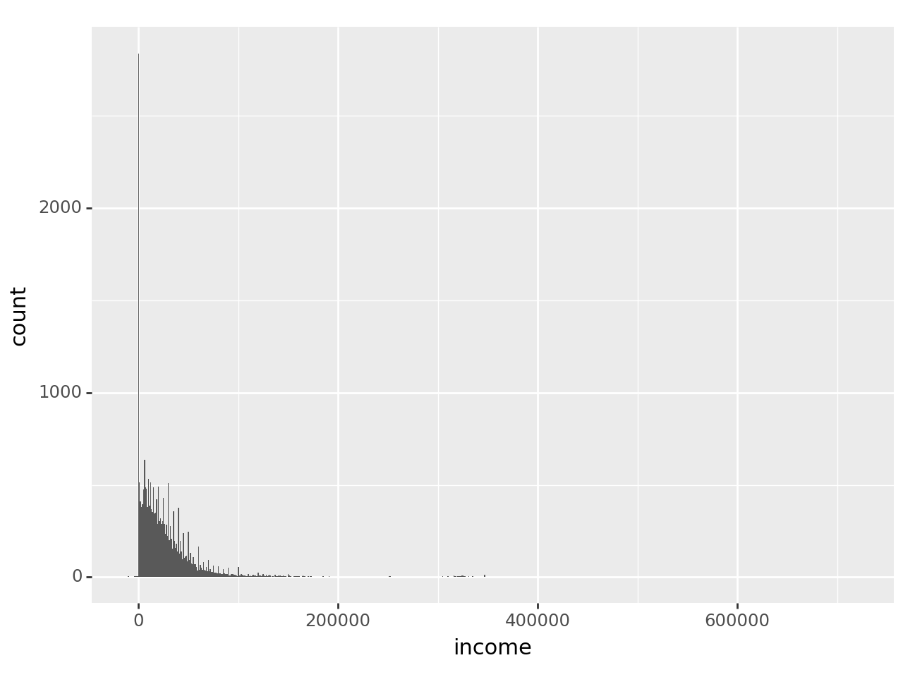

<Figure Size: (640 x 480)>

The warning about ‘non-finite values’ is just telling us that missing values were ignored, which is what we want.

The distribution certainly is skewed, to the point that it’s hard to see much. Try plotting just the incomes below $100,000 but greater than 0:

p9.ggplot(
    acs[(acs['income']<100000) & (acs['income']>0)],
    p9.aes(x = 'income')
) + p9.geom_histogram(binwidth = 1000)

<Figure Size: (640 x 480)>

Exercise

Create a histogram for age with binwidth to set 5 (years). Then create one where binwidth is set to 1 (i.e. every age gets its own bin). What do you see now that you couldn’t see before?

Solution

p9.ggplot(
    acs,
    p9.aes(x='age')
) + p9.geom_histogram(binwidth=5)

<Figure Size: (640 x 480)>

p9.ggplot(
    acs,
    p9.aes(x='age')
) + p9.geom_histogram(binwidth=1)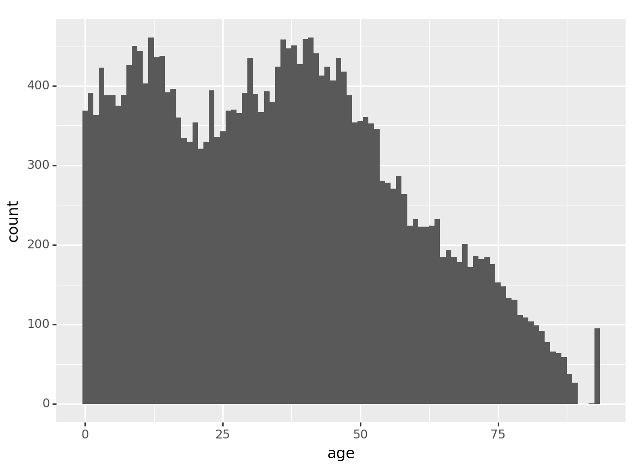

<Figure Size: (640 x 480)>

With binwidth set to 5, it’s arguably easier to see the general distribution of age. But 1 allows us to see a clear anomaly in the data: a spike on the far right. To see where it is, look at value_counts() for ages greater than 85:

acs.loc[acs['age']>85,'age'].value_counts()

age
93    95
86    64
87    59
88    38
89    27
92     1
Name: count, dtype: int64

In general, the number of people in the data set decreases with age in this age range, as one would expect. But there’s an oddly large number of people at age 93 and no one above that. The reason is that the age variable has been top-coded in this data set: 93 really means ‘93 or older’. That’s a very important piece of information if this age range is relevant to your research! You could discover it by either reading the data documentation carefully or examining the data carefully; ideally you’ll do both.

4.13.4 Categorical Variables

To examine the distribution of categorical variables, use the familiar value_counts(). Start with edu. The table will be more useful if the education categories stay in their inherent order rather than being sorted by frequency, so pass in sort=False:

acs['edu'].value_counts(sort=False)

edu
Not in universe             1123
None                        1290
Nursery school-4th grade    2500
5th-6th grade               1284
7th-8th grade               1590
9th grade                    891
10th grade                  1021
11th grade                   875
12th grade, no diploma       860
High School graduate        5763
Some college, <1 year       1495
Some college, >=1 year      3031
Associate degree            1202
Bachelor's degree           2920
Master's degree             1057
Professional degree          343
Doctorate degree             165
Name: count, dtype: int64

Things to note:

• There are no missing values, or at least none coded as such.
• The category “Not in universe” needs some investigation.
• There are more people in lower education categories than you might expect
• There may be more categories here than are useful, so you might consider combining them for analysis

There are a lot of numbers to read in that table, but a bar chart would allow you to see the patterns in it immediately. Creating one is almost identical to creating a histogram: it’s exactly the same aesthetic, but add geom_bar() instead of geom_histogram():

p9.ggplot(
    acs,
    p9.aes(x='edu')
) + p9.geom_bar()

<Figure Size: (640 x 480)>

(In this case, the warning is telling us that plotnine is using a deprecated Pandas function. Presumably the plotnine developers will change their code before it becomes a problem.)

Well that’s not very useful! There’s not enough space on the x-axis for all the labels, which is common. But this problem has a very simple solution: switch to a horizontal bar graph. All you need to do is add p9.coord_flip() to it:

p9.ggplot(
    acs,
    p9.aes(x='edu')
) + p9.geom_bar() + p9.coord_flip()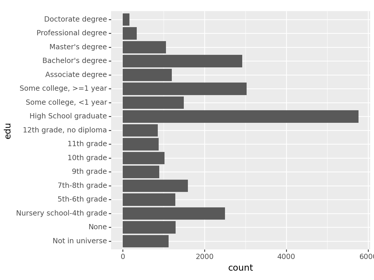

<Figure Size: (640 x 480)>

This makes horizontal the format of choice for bar graphs.

4.14 Investigate Anomalies

We’ve identified several oddities in this data set as we’ve explored it. They could have significant effects on your analysis, so it’s important to figure out what they mean.

edu has a level called ‘Not in universe.’ The Census Bureau probably isn’t actually collecting data on extra-dimensional beings, so what does this mean? Begin by examining the distribution of age for people who have ‘Not in universe’ for edu:

acs.loc[
    acs['edu']=='Not in universe',
    'age'
].describe()

count    1123.000000
mean        0.994657
std         0.807699
min         0.000000
25%         0.000000
50%         1.000000
75%         2.000000
max         2.000000
Name: age, dtype: float64

Everyone with ‘Not in universe’ for edu is under the age of three. Is the converse true?

acs.loc[acs['age']<3, 'edu'].value_counts()

edu
Not in universe             1123
High School graduate           0
Professional degree            0
Master's degree                0
Bachelor's degree              0
Associate degree               0
Some college, >=1 year         0
Some college, <1 year          0
12th grade, no diploma         0
None                           0
11th grade                     0
10th grade                     0
9th grade                      0
7th-8th grade                  0
5th-6th grade                  0
Nursery school-4th grade       0
Doctorate degree               0
Name: count, dtype: int64

People with ‘Not in universe’ are all under the age of three, and people under the age of three are always ‘Not in universe.’ It turns out that the Census Bureau uses ‘Not in universe’ to mean that the person is not in the ‘universe’ of people who were asked the question because it does not apply to them. In this case, if someone is under the age of three the Census Bureau doesn’t ask about their education. Legitimate skips are similar: questions a respondent did not answer (skipped) because they did not apply.

This is why the different coding of hispan and asian in the ATUS is somewhat puzzling: hispan is treated as a categorical variable that applies to everyone, with one valid value being ‘Not Hispanic,’ while asian is treated as a categorical variable that only applies to Asian people, with non-Asians being ‘Not in universe.’ Either way makes sense, but you’d expect them to be treated the same.

We noted more people with less than a high school education than you might expect in the United States in 2000, but that includes children who simply aren’t old enough to have graduated from high school. If we limit the sample to adults the distribution is more like what you’d expect:

acs.query('age>=18')['edu'].value_counts(sort=False)

edu
Not in universe                0
None                         291
Nursery school-4th grade     148
5th-6th grade                384
7th-8th grade                647
9th grade                    489
10th grade                   691
11th grade                   696
12th grade, no diploma       830
High School graduate        5736
Some college, <1 year       1490
Some college, >=1 year      3029
Associate degree            1202
Bachelor's degree           2920
Master's degree             1057
Professional degree          343
Doctorate degree             165
Name: count, dtype: int64

This is a good example of how you should check your work as you go: see if your data matches what you know about the population of interest, and if not, be sure there’s a valid reason why.

We also noted people with negative values for income. Who are they? Look at age, edu, and female:

acs.loc[
    acs['income']<0,
    'age'
].describe()

count    29.000000
mean     49.896552
std      13.454539
min      24.000000
25%      40.000000
50%      54.000000
75%      58.000000
max      77.000000
Name: age, dtype: float64

acs.loc[
    acs['income']<0,
    'edu'
].value_counts(sort=False)

edu
Not in universe             0
None                        0
Nursery school-4th grade    0
5th-6th grade               0
7th-8th grade               0
9th grade                   1
10th grade                  0
11th grade                  1
12th grade, no diploma      0
High School graduate        6
Some college, <1 year       3
Some college, >=1 year      6
Associate degree            5
Bachelor's degree           5
Master's degree             1
Professional degree         0
Doctorate degree            1
Name: count, dtype: int64

acs.loc[
    acs['income']<0,
    'female'
].value_counts()

female
False    16
True     13
Name: count, dtype: int64

First off, note that there are only 29 people with negative incomes, which lowers the stakes in dealing with them.

They’re all adults, but there are no other obvious patterns. One plausible explanation is that these people had losses on investments. However, in order to lose money on investments you have to have investments. So if that’s the explanation, these people may have substantial wealth even though they have negative incomes in this particular year. This is problematic if you plan to use income as a proxy for broader socio-economic status. You might consider changing negative values of income to missing.

Execise

Who are the people who marked ‘Other’ for race? (Look at the distributions of other variables for the people who have ‘Other’ for race.)

Solution

Let’s start by examining female:

acs.loc[acs['race']=='Other', 'female'].value_counts()

female
False    817
True     770
Name: count, dtype: int64

There are slightly more men than women, but not enough to matter. Next try hispanic:

acs.loc[acs['race']=='Other', 'hispanic'].value_counts()

hispanic
True     1529
False      58
Name: count, dtype: int64

Ah…almost all the people who chose ‘Other’ for race are Hispanic. What’s going on here?

To social scientists, ‘Hispanic’ is an ethnicity, and people who are Hispanic can be of different races. But to many non-specialists, Hispanic is a race like White and Black. So when some people who identified as Hispanic were asked to choose their race and did not see ‘Hispanic’ as an option, they chose ‘Other.’ The Census Bureau reworded the question in the 2010 census to try to clear this up. On the other hand, we see many researchers treat Hispanic as a race in their regression models.

4.15 Recode Values that Mean Missing to NaN

Python uses NaN to denote missing values. Functions like mean() expect that and act accordingly, typically by omitting NaN values from their calculations.

Data sets often use different codes to indicate missing values. We saw that with income: ‘BBBBBBB’ meant missing. This was automatically converted to a missing value when you converted income from a string variable to a numeric variable, but it won’t always be that simple. Recall that in the harmomized ACS produced by IPUMS, missing was coded as 9999999. It’s also common to use negative numbers to mean missing, especially -9. Functions like mean() will not recognize that 9999999 or -9 means missing and will include those values in their calculations, giving incorrect results.

The solution is to identify values that really mean missing, and then change them NaN. For example, ‘Not in universe’ for edu means missing, so change it with:

import numpy as np
acs.loc[
    acs['edu']=='Not in universe',
    'edu'
] = np.NaN
acs.loc[484]

	age	race	marital_status	edu	income	female	hispanic
person
1	33	Asian	Now married	High School graduate	16800.0	False	False
2	26	Asian	Now married	11th grade	18000.0	True	False
3	4	Asian	Never married	None	NaN	False	False
4	2	Asian	Never married	NaN	NaN	True	False

Are the negative values for income codes for missing? Take a look at them with:

acs.loc[
    acs['income']<0,
    'income'
].value_counts()

income
-10000.0    4
-4200.0     3
-200.0      2
-510.0      2
-100.0      1
-1300.0     1
-2040.0     1
-2500.0     1
-1700.0     1
-220.0      1
-4900.0     1
-8960.0     1
-3200.0     1
-550.0      1
-3800.0     1
-1600.0     1
-480.0      1
-3000.0     1
-4000.0     1
-140.0      1
-2300.0     1
-1000.0     1
Name: count, dtype: int64

The variety of values suggest these are actual quantities, not codes.

Exercise

The codebook says that for marital_status 5 means “Never married (includes under 15 years).” In other words, the Census Bureau didn’t ask about the marital status of children under the age of fifteen just like they didn’t ask about the education of children under the age of three. But for marital status they coded it as if it were known that the children were never married. Reverse this choice by changing marital_status to missing for children under fifteen.

Solution

acs.loc[
    acs['age']<15,
    'marital_status'
] = np.NaN

4.16 Examine Missing Data

Now that missing data is all coded as NaN, isna() will be True for all of it. If you do ask Python to do math with True/False, it will convert True to 1 and False to 0. So the sum of isna() is the number of observations with a missing value, which gives you a very convenient way to see how much missing data you have:

acs.isna().sum()

age                  0
race                 0
marital_status    6144
edu               1123
income            6144
female               0
hispanic             0
dtype: int64

It’s good to know you don’t have to worry about missing values for age, race, female, or hispanic, but you definitely have to think carefully about marital_status, edu, and income.

What this cannot tell you is why the data are missing. Often you can answer this question by examining the relationships between missing values and other variables. For example, what is the distribution of age for the people with missing values of income?

acs.loc[acs['income'].isna(), 'age'].describe()

count    6144.000000
mean        7.245117
std         4.315471
min         0.000000
25%         3.000000
50%         7.000000
75%        11.000000
max        14.000000
Name: age, dtype: float64

acs.loc[acs['age']<15, 'income'].describe()

count    0.0
mean     NaN
std      NaN
min      NaN
25%      NaN
50%      NaN
75%      NaN
max      NaN
Name: income, dtype: float64

It turns out that the Census Bureau did not ask about the income of children under the age of 15 just like they did not ask about their marital status, but they coded income as missing.

You should also consider relationships between missing values. In this data set, people with a missing value of income also have a missing value for marital_status because both variables were not collected for children under the age of 15. But in many data sets there are direct relationships between missing values. For example, if a subject could not be located in a wave of a survey then they may have missing values for all the variables for that survey wave.

Data is missing completely at random if the probability of it being missing is unrelated to either the observed data or the unobserved data. Thus the unobserved data has the same distribution as the observed data. Complete cases analysis (analysis of just the observed data) will have less power due to the missing data, but will be unbiased.

Data is missing at random if the probability of it being missing is related only to the observed data (the missingness is random conditional on the observed data). Thus the unobserved data can be distributed differently from the observed data. Complete cases analysis will be biased, but methods such as weighting, Blimp, or multiple imputation may be able to correct that bias–though they generally depend on being able to make inferences about the unobserved data using the observed data. For example, pollsters know people with lower levels of education are less likely to respond to polls, but they can use the responses of those people with low levels of education who do respond to make inferences about those who don’t (typically by weighting).

Data is missing not at random if the probability of it being missing is related to the unobserved data. You cannot correct for bias due to missing not at random data; worse, you can’t even detect it using the observed data. For example, UW-Madison once did a survey of its employees on the use of electronic calendars. The response rate was low and it seemed likely that people who used calendars heavily would be more motivated to respond, meaning estimates of usage would be biased high. But there was no way to know for sure if this was true since the probability of answering the survey would depend on the values of usage that were not observed.

Consider edu, which is missing for children under the age of three. If we could observe the values of edu for these children, they would probably be mostly ‘None’ with perhaps a few ‘Nursery school-4th grade’ (presumably all ‘Nursery School’). This is very different from the observed distribution of edu. This is an example of ‘missing at random’ since the probability of edu being missing depends on age and age is always observed, but it would be difficult to correct for the bias introduced because we have no actual data (just assumptions) about the distribution of edu for children under three.

Exercise

What is the likely distribution of income for people with a missing value for income? How would the mean of income change if all its missing values became known? (In other words, how do the missing values of income bias estimates of the population mean of income?)

Solution

The people who have a missing value for income are all children under the age of 15, so almost all of them presumably have zero income. Run a quick describe() on income:

acs['income'].describe()

count     21266.000000
mean      27724.104580
std       39166.397371
min      -10000.000000
25%        6000.000000
50%       18000.000000
75%       35800.000000
max      720000.000000
Name: income, dtype: float64

Note that the mean value of income in the observed data is $27,724. The mean value in the unobserved data (the children) is almost certainly much lower than that, so if their incomes were observed the full sample mean would lower. This tells us the presence of missing data makes our estimate of the mean value of income biased high.

4.17 Save Your Work

At this point the data set is reasonably clean, and what you do with it next will depend on how you plan to use it. For example, if you wanted to use education as a predictor in a regression model it would probably be wise to combine some of the categories, but if you were doing a descriptive study you might leave it as is.

If we saved the cleaned-up data as a CSV, we’d need to do a lot of work we’ve done again after loading it. Instead we’ll save the data in a format designed for saving Python objects. There are several, but pickle format is simple and easy to use. You can save a DataFrame as a pickle by calling its to_pickle() function, and you read it with the Pandas read_pickle() function. In both cases you’ll pass in the desired file name.

acs.to_pickle('acs_cleaned.pickle')

Read the data set again and you’ll see that everything is exactly how it was before you saved it:

pd.read_pickle('acs_cleaned.pickle')

		age	race	marital_status	edu	income	female	hispanic
household	person
37	1	20	White	Never married	Some college, >=1 year	10000.0	True	False
	2	19	White	Never married	Some college, >=1 year	5300.0	True	False
	3	19	Black	Never married	Some college, >=1 year	4700.0	True	False
241	1	50	White	Never married	Master's degree	32500.0	True	False
242	1	29	White	Never married	Bachelor's degree	30000.0	True	False
...	...	...	...	...	...	...	...	...
1236624	1	29	White	Now married	Some college, >=1 year	50100.0	False	False
	2	26	White	Now married	High School graduate	12000.0	True	False
1236756	1	58	White	Now married	Master's degree	69800.0	True	False
	2	61	White	Now married	Master's degree	40800.0	False	False
1236779	1	30	American Indian	Divorced	High School graduate	22110.0	False	False

27410 rows × 7 columns

In the example files you’ll find acs.pickle. It’s the result if you get by running all the steps in this chapter, including the exercises. Hopefully your acs_cleaned.pickle file is identical to it, but we’ll use acs.pickle in subsequent chapters just in case.

Remember, a pickle file can include malicious code. You don’t have to worry about that with pickle files you create, but never trust a strange pickle!

4.18 Review

As a review, here are the first steps you should take with your data. Many of them are very quick; and the ones that take more time are especially valuable. Do not skip these steps!

Read the Documentation

Identify the Variables

Look at the Data

Set the Indexes and Identify the Structure of the Data

Get Rid of Data You Won’t Use

Change Variable Names

Convert Strings Containing Numbers to Numbers

Identify the Type of Each Variable

Recode Indicator Variables

Define Categories for Categorical Variables

Examine Variable Distributions

Investigate Anomalies

Recode Values that Mean Missing to NaN

Examine Missing Data