3 Linearity
What this assumption means: The residuals have mean zero for every value of the fitted values and of the predictors. This means that relevant variables and interactions are included in the model, and the functional form of the relationship between the predictors and the outcome is correct.
Why it matters: Any association between the residuals and fitted values or predictors implies unobserved confounding (i.e., endogeneity), and no causal interpretation can be drawn from the model.
How to diagnose violations: Visually inspect a plot of residuals against fitted values and assess whether the mean of the residuals is zero at every value of \(x\), and use the RESET to test for misspecification.
How to address it: Modify the model, fit a generalized linear model, or otherwise account for endogeneity (e.g., instrumental variables analysis).
3.1 Example Model
If you have not already done so, download the example dataset, read about its variables, and import the dataset into Stata.
Then, use the code below to fit this page’s example model.
use acs2019sample, clear
reg income age commute_time i.education
Source | SS df MS Number of obs = 2,316
-------------+---------------------------------- F(7, 2308) = 59.74
Model | 1.0966e+12 7 1.5665e+11 Prob > F = 0.0000
Residual | 6.0517e+12 2,308 2.6221e+09 R-squared = 0.1534
-------------+---------------------------------- Adj R-squared = 0.1508
Total | 7.1483e+12 2,315 3.0878e+09 Root MSE = 51206
-------------------------------------------------------------------------------------
income | Coefficient Std. err. t P>|t| [95% conf. interval]
--------------------+----------------------------------------------------------------
age | 701.7906 71.27781 9.85 0.000 562.0154 841.5659
commute_time | 285.6097 48.33727 5.91 0.000 190.8207 380.3987
|
education |
High school | 10493.04 4851.444 2.16 0.031 979.3943 20006.68
Some college | 17310.86 4987.425 3.47 0.001 7530.554 27091.16
Associate's degree | 19714.38 5320.789 3.71 0.000 9280.357 30148.41
Bachelor's degree | 37524.88 5020.907 7.47 0.000 27678.92 47370.84
Advanced degree | 63986.46 5691.064 11.24 0.000 52826.32 75146.59
|
_cons | -7496.678 5166.291 -1.45 0.147 -17627.73 2634.379
-------------------------------------------------------------------------------------3.2 Statistical Tests
Use the Ramsey Regression Equation Specification Error Test (RESET) to detect specification errors in the model. It was also created in 1968 by a UW-Madison student for his dissertation! The RESET performs a nested model comparison with the current model and the current model plus some polynomial terms, and then returns the result of an F-test. The idea is, if the added non-linear terms explain variance in the outcome, then there is a specification error of some kind, such as the failure to include some curvilinear term or the use of a general linear model where a generalized linear model should have been used.
A significant p-value from the test is not an indication to thoughtlessly add several polynomial terms. Instead, it is an indication that we need to further investigate the relationship between the predictors and the outcome.
To perform the RESET, run estat ovtest. The default is to test the addition of squared, cubed, and quartic fitted values.
estat ovtestRamsey RESET test for omitted variables
Omitted: Powers of fitted values of income
H0: Model has no omitted variables
F(3, 2305) = 5.16
Prob > F = 0.0015Considering our original formula of income age commute_time i.education, we could reproduce the default of estat ovtest as,
reg income age commute_time i.education
est sto mod1

predict yhat
gen yhat2 = yhat^2
gen yhat3 = yhat^3
gen yhat4 = yhat^4

reg income age commute_time i.education yhat2 yhat3 yhat4
est sto mod2

ftest mod1 mod2
Source | SS df MS Number of obs = 2,316
-------------+---------------------------------- F(7, 2308) = 59.74
Model | 1.0966e+12 7 1.5665e+11 Prob > F = 0.0000
Residual | 6.0517e+12 2,308 2.6221e+09 R-squared = 0.1534
-------------+---------------------------------- Adj R-squared = 0.1508
Total | 7.1483e+12 2,315 3.0878e+09 Root MSE = 51206
-------------------------------------------------------------------------------------
income | Coefficient Std. err. t P>|t| [95% conf. interval]
--------------------+----------------------------------------------------------------
age | 701.7906 71.27781 9.85 0.000 562.0154 841.5659
commute_time | 285.6097 48.33727 5.91 0.000 190.8207 380.3987
|
education |
High school | 10493.04 4851.444 2.16 0.031 979.3943 20006.68
Some college | 17310.86 4987.425 3.47 0.001 7530.554 27091.16
Associate's degree | 19714.38 5320.789 3.71 0.000 9280.357 30148.41
Bachelor's degree | 37524.88 5020.907 7.47 0.000 27678.92 47370.84
Advanced degree | 63986.46 5691.064 11.24 0.000 52826.32 75146.59
|
_cons | -7496.678 5166.291 -1.45 0.147 -17627.73 2634.379
-------------------------------------------------------------------------------------
(option xb assumed; fitted values)
(2,684 missing values generated)
(2,684 missing values generated)
(2,684 missing values generated)
(2,684 missing values generated)
Source | SS df MS Number of obs = 2,316
-------------+---------------------------------- F(10, 2305) = 43.59
Model | 1.1369e+12 10 1.1369e+11 Prob > F = 0.0000
Residual | 6.0114e+12 2,305 2.6080e+09 R-squared = 0.1590
-------------+---------------------------------- Adj R-squared = 0.1554
Total | 7.1483e+12 2,315 3.0878e+09 Root MSE = 51068
-------------------------------------------------------------------------------------
income | Coefficient Std. err. t P>|t| [95% conf. interval]
--------------------+----------------------------------------------------------------
age | 1404.129 789.7707 1.78 0.076 -144.6067 2952.864
commute_time | 545.7099 325.8935 1.67 0.094 -93.36522 1184.785
|
education |
High school | 17508.73 10572.99 1.66 0.098 -3224.843 38242.3
Some college | 31188.88 17782.55 1.75 0.080 -3682.598 66060.36
Associate's degree | 36316.61 20626.42 1.76 0.078 -4131.668 76764.89
Bachelor's degree | 74618.8 40766.96 1.83 0.067 -5324.962 154562.6
Advanced degree | 124955.8 68933.79 1.81 0.070 -10222.93 260134.5
|
yhat2 | -.000015 .0000301 -0.50 0.618 -.0000741 .000044
yhat3 | 8.16e-13 3.25e-10 0.00 0.998 -6.36e-10 6.38e-10
yhat4 | 6.36e-16 1.19e-15 0.53 0.593 -1.70e-15 2.97e-15
_cons | -27124.49 20463.84 -1.33 0.185 -67253.94 13004.97
-------------------------------------------------------------------------------------
Assumption: mod1 nested in mod2
F( 3, 2305) = 5.16
prob > F = 0.0015(Note you will need to install ftest with ssc install ftest first.)
We can add the rhs option to perform the test over the predictors instead of the fitted values. This option will add squared, cubic, and quartic terms for each predictor.
estat ovtest, rhsRamsey RESET test for omitted variables
Omitted: Powers of independent variables
H0: Model has no omitted variables
F(6, 2302) = 5.64
Prob > F = 0.00003.3 Visual Tests
Plot the residuals against the fitted values and predictors. Add a conditional mean line. If the mean of the residuals deviates from zero, this is evidence that the assumption of linearity has been violated.
First, add predicted values (yhat) and residuals (res) to the dataset.
reg income age commute_time i.education
predict yhat
predict res, residuals
Source | SS df MS Number of obs = 2,316
-------------+---------------------------------- F(7, 2308) = 59.74
Model | 1.0966e+12 7 1.5665e+11 Prob > F = 0.0000
Residual | 6.0517e+12 2,308 2.6221e+09 R-squared = 0.1534
-------------+---------------------------------- Adj R-squared = 0.1508
Total | 7.1483e+12 2,315 3.0878e+09 Root MSE = 51206
-------------------------------------------------------------------------------------
income | Coefficient Std. err. t P>|t| [95% conf. interval]
--------------------+----------------------------------------------------------------
age | 701.7906 71.27781 9.85 0.000 562.0154 841.5659
commute_time | 285.6097 48.33727 5.91 0.000 190.8207 380.3987
|
education |
High school | 10493.04 4851.444 2.16 0.031 979.3943 20006.68
Some college | 17310.86 4987.425 3.47 0.001 7530.554 27091.16
Associate's degree | 19714.38 5320.789 3.71 0.000 9280.357 30148.41
Bachelor's degree | 37524.88 5020.907 7.47 0.000 27678.92 47370.84
Advanced degree | 63986.46 5691.064 11.24 0.000 52826.32 75146.59
|
_cons | -7496.678 5166.291 -1.45 0.147 -17627.73 2634.379
-------------------------------------------------------------------------------------
(option xb assumed; fitted values)
(2,684 missing values generated)
(2,684 missing values generated)Now, plot the residuals and fitted values. Add a horizontal line with geom_hline() as the reference line, and add a conditional mean line with geom_smooth().
scatter res yhat || ///
    lowess res yhat, ///
    legend(off) ///
    yline(0, lcolor(black))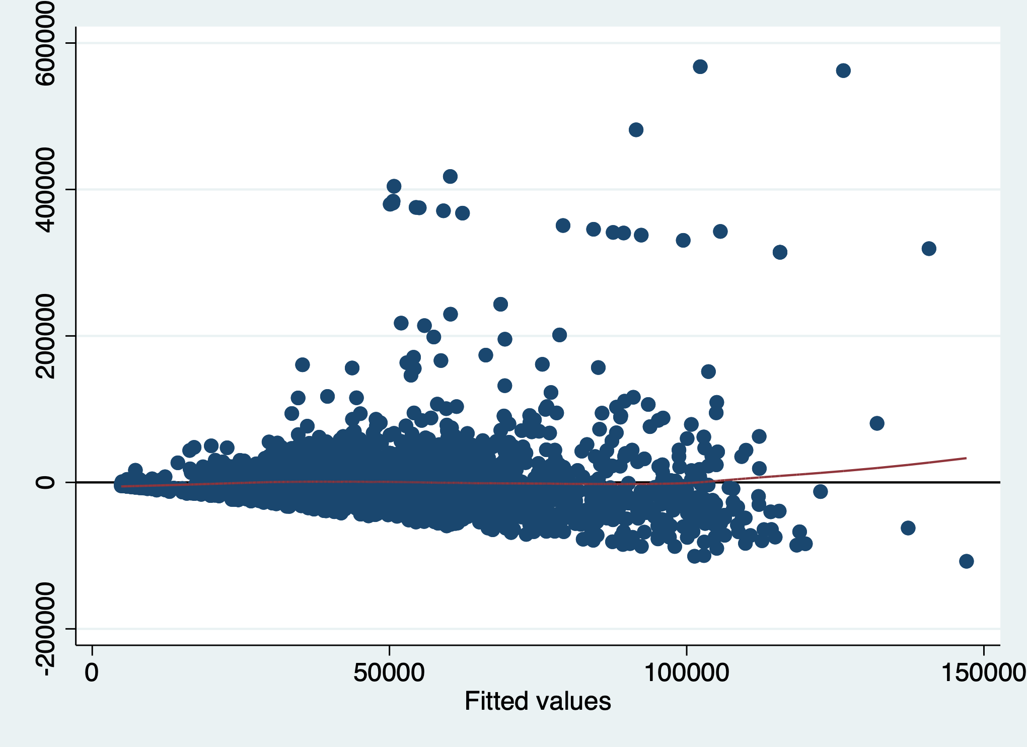
All we are looking for here is whether the conditional mean line deviates from the horizontal reference line, and the two lines overlap for the most part. Although there is an upward trend on the right, very few points exist there so some deviation is expected. Overall, it does not look like there is evidence that the assumption of linearity has been violated.
However, we should be concerned about the fan-shaped residuals that increase in variance from left to right. This is discussed in the chapter on homoscedasticity.
We must also check the residuals against each of the predictors. We will just check age here.
scatter res age || ///
    lowess res age, ///
    legend(off) ///
    yline(0, lcolor(black))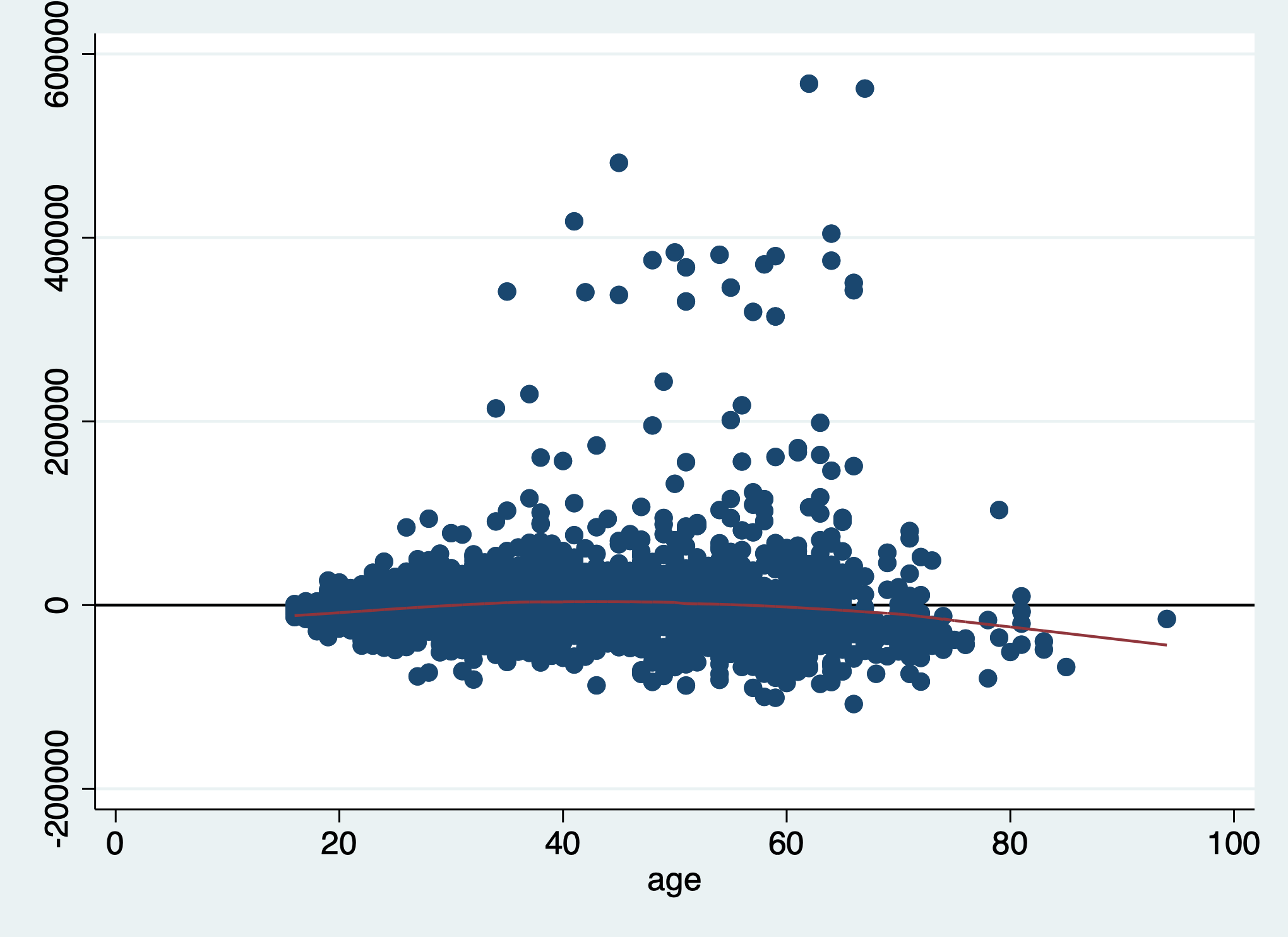
The mean of the residuals is negative on the left, positive in the middle, and again negative on the right. There is evidence for non-linearity with respect to the age variable.
Now, check the residual variance against a categorical predictor, education.
Adding a conditional mean line with a categorical variable requires us to treat the variable as numeric:
scatter res education || ///
    lowess res education, ///
    legend(off) ///
    yline(0, lcolor(black))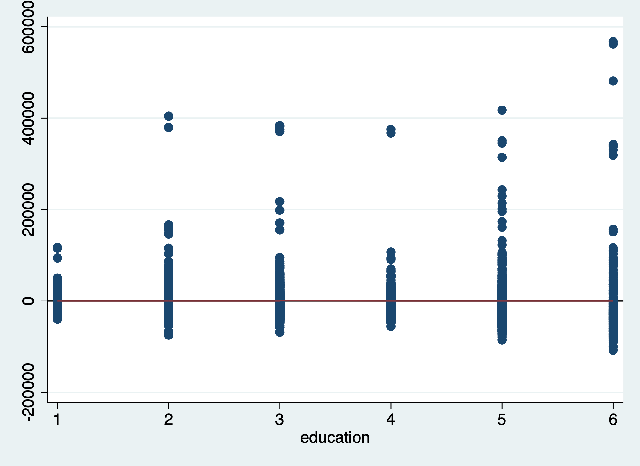
This plot looks good. The mean of the residuals looks to be exactly zero for every level of education.
Optionally, we can also plot the residuals against other variables not included in the model, to see if they correlate with the residuals.
We can try plotting the residuals against hours_worked, which was not in the model.
scatter res hours_worked || ///
    lowess res hours_worked, ///
    legend(off) ///
    yline(0, lcolor(black))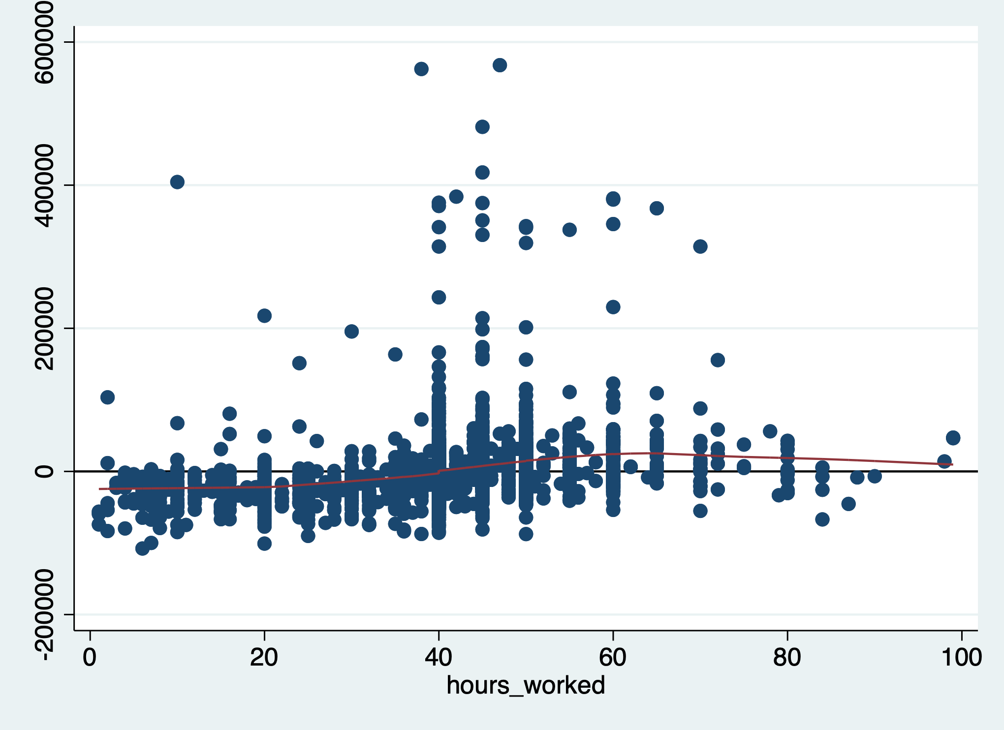
The conditional mean increases from left to right, suggesting a positive relationship. If we have a good theoretical reason to include this variable in our model, we could add it.
3.4 Corrective Actions
We can address non-linearity in one or more ways:
- Check the other regression assumptions, since a violation of one can lead to a violation of another.
- Modify the model formula by adding or dropping variables or interaction terms.
- Do not simply add every possible variable and interaction in an attempt to explain more variance. Carelessly adding variables can introduce suppressor effects or collider bias.
- Add polynomial terms to the model (squared, cubic, etc.).
- Fit a generalized linear model.
- Fit an instrumental variables model in order to account for the correlation of the predictors and residuals.
After you have applied any corrections or changed your model in any way, you must re-check this assumption and all of the other assumptions.