clear all
use https://sscc.wisc.edu/sscc/pubs/stata_dates/dates.dtaWorking with Dates and Times in Stata
This article will introduce you to working with dates and times in Stata. We won’t cover all the details–this is a topic with a lot of details–but what we will cover has a good chance of being all you’ll need.
You’ll retain more of what you learn from this article if you run the example code yourself and try the exercises. To set up, open Stata, clear out anything you were doing before, and load the first example data set from the SSCC’s web server:
Note: this article was written as a Jupyter Notebook using the nbstata kernel and then converted to HTML by Quarto. You’ll notice a few bits of Stata code that are only needed to make that process work well, such as using the ab(30) option with list to prevent variable names from being abbreviated. You don’t need to copy them. You probably want to use the data browser to look at the data anyway.
Converting Dates and Times
Often your first task is to convert the dates and times in your data set to Stata format, and most of the time everything after that is easy.
How Stata Stores Dates and Times
Stata stores a date as a number: most commonly the number of days that have passed since January 1, 1960. Thus 23,056 means February 15th, 2023. But the time unit could also be weeks, months, quarters, etc., depending on what’s convenient for your project. When you need to store a date and time (a datetime), the time unit becomes milliseconds. Thus 1,992,047,400,000 means 2:30PM on February 15th, 2023. Note that this number is too big to store accurately using the default float variable type. Always use double precision numbers for datetime variables.
Storing dates as numbers of time units since January 1, 1960 means you can do math with them. For example, if you know a subject’s birthday and the date of the beginning of the study, you can calculate how old they were when the study began by just subtracting. But dates as numbers of time units don’t mean much to most humans. Fortunately, there are special formats for dates that tell Stata to display those numbers as the corresponding human-readable date. These formats all start with %t followed by a letter corresponding to the time unit: %td for days, %tw for weeks, %tm for months, %tq for quarters, etc. The format for datetime variables is called %tc (think ‘clock’).
If a variable contains 23,056 and has been formatted with %td, it will be displayed as 15feb2023. But if it’s formatted with %tm it will be displayed as 3881m5, meaning month 5 (May) of the year 3881. The date is much later becuase it’s now assumed to be 23,056 months after January 1960 rather than 23,056 days. It’s really the format that determines what the time unit is.
To create a Stata date variable, you’ll choose a time unit, convert the date to “number of that time unit that have passed since January 1, 1960”, and then apply the appropriate format. The second step in that process is the tricky one but Stata has a variety of functions that will do it for you, depending on the time unit you want and how the date is currently stored.
Note that Excel stores dates as the number of days since January 1, 1900 and some other systems use January 1, 1970. Be careful about converting dates from other programs. If you are planning to make data widely available or to store it for a long time, consider storing dates as separate numbers for year, month, day, etc. as that form is easy to convert and unambiguous.
Converting Numbers to Dates
Because date components stored as separate numbers are easy to use, they’re very common. The nd (numeric date) variables in the example data set are in this form:
list nd*, ab(30)
     +------------------------------------------------------------------+
     | nd_day   nd_month   nd_year   nd_hours   nd_minutes   nd_seconds |
     |------------------------------------------------------------------|
  1. |     15          2      2023          2           30           30 |
     +------------------------------------------------------------------+
The mdy() function converts numbers for month, day, and year to dates with day as the time unit. The arguments can be either numbers or variables containing numbers, and the name of the function tells you the order they go in: month, day, and then year. Thus:
gen nd = mdy(nd_month, nd_day, nd_year)
list nd
     +-------+
     |    nd |
     |-------|
  1. | 23056 |
     +-------+
To make this readable, apply the %td format to the nd variable:
format %td nd
list nd
     +-----------+
     |        nd |
     |-----------|
  1. | 15feb2023 |
     +-----------+
TipExercise
The variables year_of_birth, month_of_birth, and day_of_birth contain the birthdate of a (made up) subject. Convert it to Stata form with a human-readable format.
NoteSolution
gen birthdate = mdy(month_of_birth, day_of_birth, year_of_birth)
format birthdate %td
list birthdate
     +-----------+
     | birthdate |
     |-----------|
  1. | 19sep1975 |
     +-----------+
To create a date where month is the time unit, use the ym() function. Again, the function name tells you the order of the arguments: year and then month. The other conversion functions follow the same pattern: yq() takes year and then quarter and converts them to a date with quarters as the time unit, etc.
To make a date variable where the time unit is month readable, apply the %tm format.
Thus to convert nd to a monthly date, run:
gen nd_monthly = ym(nd_year, nd_month)
format nd_monthly %tm
list nd_monthly, ab(30)
     +------------+
     | nd_monthly |
     |------------|
  1. |     2023m2 |
     +------------+
TipExercise
Often you’ll find data sets only contain birth month and birth year, to preserve anonymity. Convert year_of_birth and month_of_birth to a monthly variable.
NoteSolution
gen birthmonth = ym(year_of_birth, month_of_birth)
format birthmonth %tm
list birthmonth, ab(30)
     +------------+
     | birthmonth |
     |------------|
  1. |     1975m9 |
     +------------+
To create datetime variables, you can use the mdyhms() function, where hms means hours, minutes, and seconds. Use gen double to create the new variable as a double precision variable so it can store time accurately.
gen double nd_time = mdyhms(nd_month, nd_day, nd_year, nd_hours, nd_minutes, nd_seconds)
format nd_time %tc
list nd_time
     +--------------------+
     |            nd_time |
     |--------------------|
  1. | 15feb2023 02:30:30 |
     +--------------------+
TipExercise
Repeat the steps above, but don’t specify that the new variable be of type double (i.e. run gen nd_time2 = ... rather than gen double nd_time2 = ...). What goes wrong and why?
NoteSolution
gen nd_time2 = mdyhms(nd_month, nd_day, nd_year, 8, 0, 0)
format nd_time2 %tc
list nd_time2
     +--------------------+
     |           nd_time2 |
     |--------------------|
  1. | 15feb2023 08:00:52 |
     +--------------------+
Without gen double, the nd_time2 variable is created as the default variable type, float. float has about seven digits of accuracy (compared to sixteen for double), which is not enough to store time in milliseconds precisely. The result is a rounding error of 52 seconds (about 52,000 milliseconds). Always use double for datetime variables!
Converting Strings to Dates
It’s also common to have dates stored as strings (text). Again, there are a variety of functions available for converting such strings to dates, depending on the time unit desired. The date() function converts strings to dates with days as the time unit; weekly(), monthly(), etc. convert to longer time units, and clock() converts to datetime.
For all of these functions the first argument is a a string or variable containing strings with the date to be converted. The second argument is a string called a mask that tells the function what date/time components the string contains and in what order. For example, the mask "MDY" means “month, day, year.” These functions are impressively intelligent about identifying components and their meaning. For example, the mask "MDY" will work for both February 15, 2023 and 2/15/2023. It will work on a variety of abbreviations for the month name as well.
The following components can be used in a mask (from the Stata help file for dates):
| Component | Meaning |
|---|---|
| D | day |
| W | week |
| M | month |
| Q | quarter |
| H | half-year |
| Y | year |
| 19Y | two-digit year in the 1900s |
| 20Y | two-digit year in the 2000s |
| h | hour |
| m | minute |
| s | second |
| # | placeholder for something to be ignored |
Consider the dates sd1, sd2, and sd3:
list sd1 sd2 sd3
     +---------------------------------------+
     |          sd1         sd2          sd3 |
     |---------------------------------------|
  1. | Feb. 15 2023   2/15/2023   2023-02-15 |
     +---------------------------------------+
sd1 and sd2 are both in the form month, day, year, so they can both be converted using the mask "MDY":
gen sd1_date = date(sd1, "MDY")
gen sd2_date = date(sd2, "MDY")
format sd1_date sd2_date %td
list sd1_date sd2_date
     +-----------------------+
     |  sd1_date    sd2_date |
     |-----------------------|
  1. | 15feb2023   15feb2023 |
     +-----------------------+
sd3 is in ISO standard format: year, month, day. Thus it needs the mask "YMD":
gen sd3_date = date(sd3, "YMD")
format sd3_date %td
list sd3_date
     +-----------+
     |  sd3_date |
     |-----------|
  1. | 15feb2023 |
     +-----------+
TipExercise
interview contains the date on which the fictional subject was interviewed. Convert it to a Stata date.
NoteSolution
gen interview_date = date(interview, "DMY")
format interview_date %td
list interview_date, ab(30)
     +----------------+
     | interview_date |
     |----------------|
  1. |      01may2005 |
     +----------------+
The string sd4 contains just a month and year:
list sd4
     +----------+
     |      sd4 |
     |----------|
  1. | Feb 2023 |
     +----------+
Converting it calls for the monthly() function with the mask "MY" and the %tm format:
gen sd4_date = monthly(sd4, "MY")
format sd4_date %tm
list sd4_date
     +----------+
     | sd4_date |
     |----------|
  1. |   2023m2 |
     +----------+
Masks for the the conversion functions of larger time units (weekly(), monthly(), etc.) can only contain the time unit and a year. For them, all the mask really does is specify the order they appear in.
To convert datetime variables use the clock() function–and usually a longer mask. Consider sd5:
list sd5
     +---------------------+
     |                 sd5 |
     |---------------------|
  1. | 2023-02-15 14:30:00 |
     +---------------------+
The date components are year, month, day, hours, minutes, and seconds, so the mask is "YMDhms". Don’t forget to use a double precision variable!
gen double sd5_datetime = clock(sd5, "YMDhms")
format sd5_datetime %tc
list sd5_datetime
     +--------------------+
     |       sd5_datetime |
     |--------------------|
  1. | 15feb2023 14:30:00 |
     +--------------------+
Now consider sd6:
list sd6
     +----------------------------+
     |                        sd6 |
     |----------------------------|
  1. | 2:30PM on February 15, '23 |
     +----------------------------+
The date components here are hours, minutes, month, day, and year. But there are some complications:
You might be worried about the hour, but Stata will automatically detect the “PM” and take it into account.
The word “on” is not a date component. You need to tell Stata to ignore it by putting # in the mask between minute and month, meaning the element there should be ignored.
The year is only two digits. Use 20Y to tell Stata to assume it’s 2023 rather than 1923.
There’s no information about seconds. That’s okay: Stata will assume the seconds should be zero. If something like day or month is missing, Stata will assume it should be one.
gen double sd6_datetime = clock(sd6, "hm#MD20Y")
format sd6_datetime %tc
list sd6_datetime
     +--------------------+
     |       sd6_datetime |
     |--------------------|
  1. | 15feb2023 14:30:00 |
     +--------------------+
What if you only cared about the date of sd6 and not the time? Just use the date() function and tell it to ignore all the time elements:
gen sd6_date = date(sd6, "###MD20Y")
format sd6_date %td
list sd6_date
     +-----------+
     |  sd6_date |
     |-----------|
  1. | 15feb2023 |
     +-----------+
However, you cannot use the same approach to convert sd6 to a monthly date. Remember the mask for functions like monthly() is much simpler and does not include # to ignore elements. You’ll learn an alternative method shortly.
TipExercise
interview_time contains the time the subject was interviewed on the date contained in interview. Combine the two strings and convert them to a single datetime variable.
NoteSolution
You could create a new variable to hold the combination of interview and interview_time, but you can also just pass them to clock directly.
gen double interview_datetime = clock(interview + interview_time, "DMYhm")
format interview_datetime %tc
list interview_datetime
     +--------------------+
     | interview_datetime |
     |--------------------|
  1. | 01may2005 10:15:00 |
     +--------------------+
Note that the combined string has no separator between year and hour:
display interview + interview_time1 May, 200510:15AMThat’s okay: Stata is smart enough to know that 2005 is a year and what follows must be the hour.
Converting Between Date Formats
You can convert dates from one format to another using one of a set of conversion functions. For example, to convert sd1_date from a regular date with days as the time unit to a monthly date, use the mofd() function.
gen sd1_monthly = mofd(sd1_date)
format sd1_monthly %tm
list sd1_date sd1_monthly, ab(30)
     +-------------------------+
     |  sd1_date   sd1_monthly |
     |-------------------------|
  1. | 15feb2023        2023m2 |
     +-------------------------+
For mofd() think “months of days” as in “make months out of days.” Similar functions include dofm() (days of months), wofd() (weeks of days), dofc() (days of clock, as in datetime), etc.
Note how in converting sd1_date to sd1_monthly the day of the month was lost. If you convert back, Stata will fill in one for the day:
gen sd1_date2 = dofm(sd1_monthly)
format sd1_date2 %td
list sd1_date sd1_monthly sd1_date2, ab(30)
     +-------------------------------------+
     |  sd1_date   sd1_monthly   sd1_date2 |
     |-------------------------------------|
  1. | 15feb2023        2023m2   01feb2023 |
     +-------------------------------------+
This is just like filling in missing components when reading in a date: Stata will fill in a one or zero as appropriate.
We previously converted sd6 to a date even though it contained time components by telling the date() function to ignore them, but noted that we could not convert it to monthly the same way. One solution is to first create sd6_date as a daily date and then convert it to monhtly. But note that you can combine those steps:
gen sd6_monthly = mofd(date(sd6, "###MD20Y"))
format sd6_monthly %tm
list sd6 sd6_monthly, ab(30)
     +------------------------------------------+
     |                        sd6   sd6_monthly |
     |------------------------------------------|
  1. | 2:30PM on February 15, '23        2023m2 |
     +------------------------------------------+
TipExercise
Convert sd1_date to a quarterly date.
NoteSolution
If you didn’t run the example code that created sd1_date, start with:
gen sd1_date = date(sd1, "MDY")
format sd1_date %td
Now convert it to quarterly:
gen sd1_quarterly = qofd(sd1_date)
format sd1_quarterly %tq
list sd1_date sd1_quarterly, ab(30)
     +---------------------------+
     |  sd1_date   sd1_quarterly |
     |---------------------------|
  1. | 15feb2023          2023q1 |
     +---------------------------+
February is in the first quarter of the year.
Using Dates
Once you have your dates in Stata format, they’re easy to use–but they do take some getting used to. Keep in mind that they are really numbers, and you can do things with them that make sense for numbers.
The data set claims.dta contains initial claims (ICSA) for unemployment insurance on a weekly basis from January 2015 to February 2023. This is a key measure of the state of job market: high numbers of claims means many people have been laid off from their jobs. The data set was obtained from the Federal Reserve Economic Database (FRED) using the import fred command. You need to make an account with FRED and obtain a key to use that command, and if you’re interested in the US economy you probably want to do that.
The variable daten is the date in Stata format. Note that it’s a daily date (the format is %td) even though there’s one observation per week. The variable dates is the date in string format. Since daten is just a number, you can do things like use it in graphs:
clear
use https://sscc.wisc.edu/sscc/pubs/stata_dates/claims
line ICSA daten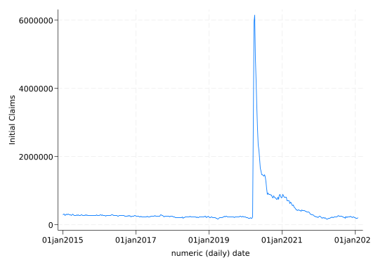
Yes, that massive spike is the effect of the COVID-19 pandemic.
Date Conditions and Constants
Suppose we wanted to divide this dataset into the pre-pandemic period and the post-pandemic period, creating an indicator for “post-pandemic.” We’ll call March 15th, 2020, the start of the pandemic for our purposes, since that’s when it began to clearly impact the job market.
Conceptually, we want to set post to the condition “daten is after March 15th, 2020” (i.e. it will get a 1 if that condition is true and a 0 if that condition is false). But how to we code that condition in Stata?
Since dates are stored as number of days since January 1, 1960, “before” and “after” can be done with less than and greater than, respectively. But that means we need “March 15th, 2020” as a number of days since January 1 1960 just like daten. You can do that using the same conversion functions used to convert variables into dates, just passing in constants instead of variables. I would suggest that mdy() is the easiest to use:
gen post = (daten > mdy(3, 15, 2020))
TipExercise
Suppose we declare (somewhat arbitrarily) that the pandemic’s intensive period ended on June 1st, 2021. Create an indicator variable called pandemic that is 1 for weeks during the intensive period and 0 outside it. Find the mean value of ICSA for both periods.
NoteSolution
gen pandemic = (daten > mdy(3, 15, 2020)) & (daten < mdy(6, 1, 2021))
table pandemic, stat(mean ICSA)
--------------------
         |      Mean
---------+----------
pandemic |
  0      |  246338.9
  1      |   1313667
  Total  |  405302.6
--------------------
Don’t let the alignment of those numbers fool you: the mean is MUCH higher in the pandemic period. (Yes, we could fix the table’s alignment if we wanted to–the table command is meant for building publication-quality tables as well as easy but useful ones.)
Date Components
The year() function will extract the year from a date as a simple number:
gen year = year(daten)
list daten year in 1/5
     +------------------+
     |     daten   year |
     |------------------|
  1. | 03jan2015   2015 |
  2. | 10jan2015   2015 |
  3. | 17jan2015   2015 |
  4. | 24jan2015   2015 |
  5. | 31jan2015   2015 |
     +------------------+
Similar functions exist for other time components, such as month() and quarter(). However, these functions only work with daily dates–they assume that the date they’re given is number of days since January 1, 1960. That’s not a problem though: just convert whatever you have to a daily date with the appropriate conversion function, like dofm() or dofc().
TipExercise
Create a variable containing the quarter of each observation. Which quarter has the highest average number of claims? How does that change if you exclude the pandemic period?
NoteSolution
gen quarter = quarter(daten)
table quarter, stat(mean ICSA)
-------------------
        |      Mean
--------+----------
quarter |
  1     |  370611.1
  2     |  580634.6
  3     |  361885.7
  4     |  311632.1
  Total |  405302.6
-------------------
table quarter if !pandemic, stat(mean ICSA)
-------------------
        |      Mean
--------+----------
quarter |
  1     |  229354.8
  2     |    246378
  3     |  265706.5
  4     |    244129
  Total |  246338.9
-------------------
The massive spike in claims in the second quarter of 2020 gives quarter 2 the highest average for the entire period, but if you exclude the pandemic period quarter 3 is higher.
Date Arithmetic and Durations
Now load a small selection from the American Time Use Survey (ATUS):
clear
use https://sscc.wisc.edu/sscc/pubs/stata_dates/atus
set linesize 120
list in 1/5
     +------------------------------------------------------------------------------+
     |         caseid   actline                                 activity   duration |
     |------------------------------------------------------------------------------|
  1. | 20170101170002         1                                 Sleeping         90 |
  2. | 20170101170002         2   Washing, dressing and grooming oneself         30 |
  3. | 20170101170002         3                Travel related to working         15 |
  4. | 20170101170002         4          Waiting associated with working         15 |
  5. | 20170101170002         5                           Work, main job        150 |
     +------------------------------------------------------------------------------+
The ATUS asks subjects to list all their activities for a 24 hour period starting at 4:00AM the previous day. The ATUS gives the duration of each activity, but let’s use that to calculate the start and end time of each activity. While we’ll be working with times in this example, if we had durations measured in days and wanted to talk about start and end dates the process would be almost identical.
The start and end times will need to be stored as datetime variables, but we don’t know the exact date the subjects were interviewed. That’s okay: we’ll just ignore the date part of the datetimes. They’ll all end up being times on January 1, 1960 or January 2nd, 1960 (since the activity list continues until 4:00AM the next day) which you can just think of as “Day One” and “Day Two.”
Since datetimes are just numbers, if you have a starting time and add the duration to it, the result will be the end time. But they do all need to be in the same units. Datetimes are in milliseconds, so the first thing to do is calculate the duration of each activity in milliseconds. To do so multiply by 60 (60 seconds per minute) and then 1000 (1000 milliseconds per second):
gen double dur_ms = duration * 60 * 1000The start time of the first activity for each person is 4:00AM. Recall that _n is the observation number of the current observation, so the condition if _n==1 identifies the first observation. If the command starts with by caseid: that will be the first observation for each person, but since the data are not sorted by casedid (yet) make that bysort caseid:. The hms() function allows us to easily specify a time in terms of ours, minutes and seconds:
bysort caseid: gen double start = hms(4, 0, 0) if _n==1(3,977 missing values generated)For all the other activities, their start time is the start time of the previous activity plus the duration of the previous activity in milliseconds:
by caseid: replace start = start[_n-1] + dur_ms[_n-1] if _n>1(3977 real changes made)Recall that putting square brackets after a variable allows us to access the value of the variable for a given observation number. Since _n is the current observation, start[_n-1] means “the value of start for the observation before the current observation.”
The end time for every activity is its start time plus its duration:
gen double end = start + dur_msNow all you need to do is format start and end appropriately to see the results:
format start end %tc
list caseid actline duration start end in 1/5
     +-------------------------------------------------------------------------------+
     |         caseid   actline   duration                start                  end |
     |-------------------------------------------------------------------------------|
  1. | 20170101170002         1         90   01jan1960 04:00:00   01jan1960 05:30:00 |
  2. | 20170101170002         2         30   01jan1960 05:30:00   01jan1960 06:00:00 |
  3. | 20170101170002         3         15   01jan1960 06:00:00   01jan1960 06:15:00 |
  4. | 20170101170002         4         15   01jan1960 06:15:00   01jan1960 06:30:00 |
  5. | 20170101170002         5        150   01jan1960 06:30:00   01jan1960 09:00:00 |
     +-------------------------------------------------------------------------------+
Note that if you were given start and end times you could easily calculate duration. Just remember it will start out as duration in milliseconds so you probably want to convert it to something more convenient, like minutes:
gen duration2 = (end - start) / 60 / 1000
list caseid actline duration duration2 in 1/5, ab(30)
     +-------------------------------------------------+
     |         caseid   actline   duration   duration2 |
     |-------------------------------------------------|
  1. | 20170101170002         1         90          90 |
  2. | 20170101170002         2         30          30 |
  3. | 20170101170002         3         15          15 |
  4. | 20170101170002         4         15          15 |
  5. | 20170101170002         5        150         150 |
     +-------------------------------------------------+
Our final example won’t actually introduce anything new about dates, so feel free to stop here if that’s your main goal in reading this. Continue if you want more practice with dates, more practice restructuring data, or need to do something similar to the final example.
Restructuring Date-Based Data
The ATUS has one observation per subject per activity, but for some puroposes it’s better to break the day up into blocks of time and have one observation per person per time block. That makes it much easier to say “What was the subject doing at noon?” It could also allow you to create a model for how the person chooses to spend each time block.
We’ll convert this data set to one where each subject has one row for each 15 minute time block. If a subject does two or more activities in a time block, we’ll assign the block to the activity they spent the most time on, or if that’s a tie to the one they did first. The overall plan is:
- Expand the data set so there’s one observation per minute (since the durations are in minutes)
- Identify which time block each minute belongs to
- Identify the activity we want to assign the block to
- Drop all but one observation per time block
First, use the expand command to make a copy of each activity for each minute that it lasted:
expand duration(283,823 observations created)We use the duration variable to tell expand how many copies to make. The first observation has a duration of 90, so there are now 90 copies of that observation. (You can also use just a number with expand, for example expand 10 to make 10 copies of each observation.)
Now we need to associate each observation with a different minute. Since the first activity starts at 4:00AM, the first observation for that activity should be for 4:00AM, the second should be 4:01AM, the third 4:02AM, etc. This time is the start time plus one minute per observation number minus one (since the first observation is 4:00AM and not 4:01AM). Don’t forget to convert minutes to milliseconds. Also, this needs to be done separately for each activity (i.e. observation numbers need to start over from 1 for every activity):
bysort caseid actline: gen double time = start + (_n-1)*60*1000
format time %tc

list caseid actline activity start time in 1/5, ab(30)
     +-------------------------------------------------------------------------------+
     |         caseid   actline   activity                start                 time |
     |-------------------------------------------------------------------------------|
  1. | 20170101170002         1   Sleeping   01jan1960 04:00:00   01jan1960 04:00:00 |
  2. | 20170101170002         1   Sleeping   01jan1960 04:00:00   01jan1960 04:01:00 |
  3. | 20170101170002         1   Sleeping   01jan1960 04:00:00   01jan1960 04:02:00 |
  4. | 20170101170002         1   Sleeping   01jan1960 04:00:00   01jan1960 04:03:00 |
  5. | 20170101170002         1   Sleeping   01jan1960 04:00:00   01jan1960 04:04:00 |
     +-------------------------------------------------------------------------------+
The next step is to identify the 15-minute block each observation falls into. Dividing time by 15 minutes and throwing away the remainder would give you blocks identified by number (i.e. block 0, block 1, etc.) For some purposes that might be what you want. But for this example we’ll multiply by 15 minutes again so the identifier is the time the block starts:
gen double time_block = int(time/(15*60*1000)) * 15*60*1000
format time_block %tc
list caseid actline time time_block in 1/5
     +--------------------------------------------------------------------+
     |         caseid   actline                 time           time_block |
     |--------------------------------------------------------------------|
  1. | 20170101170002         1   01jan1960 04:00:00   01jan1960 04:00:00 |
  2. | 20170101170002         1   01jan1960 04:01:00   01jan1960 04:00:00 |
  3. | 20170101170002         1   01jan1960 04:02:00   01jan1960 04:00:00 |
  4. | 20170101170002         1   01jan1960 04:03:00   01jan1960 04:00:00 |
  5. | 20170101170002         1   01jan1960 04:04:00   01jan1960 04:00:00 |
     +--------------------------------------------------------------------+
Our chosen data structure can only have one activity per 15 minute block, and we’ve chosen to keep the one that they spent the most time on, or the activity they did first in case of a tie. So we need to identify how much time the subject spent on each activity during each block. (We don’t care that they spent two hours sleeping if only one minute of it falls in the block we’re looking at.)
Since each observation represents one minute, _N, the number of observations, will tell us how many minutes they spent on an activity if we look at each activity within a block separately:
bysort caseid time_block actline: gen minutes = _N
list caseid actline activity time_block minutes in 1/5
     +--------------------------------------------------------------------+
     |         caseid   actline   activity           time_block   minutes |
     |--------------------------------------------------------------------|
  1. | 20170101170002         1   Sleeping   01jan1960 04:00:00        15 |
  2. | 20170101170002         1   Sleeping   01jan1960 04:00:00        15 |
  3. | 20170101170002         1   Sleeping   01jan1960 04:00:00        15 |
  4. | 20170101170002         1   Sleeping   01jan1960 04:00:00        15 |
  5. | 20170101170002         1   Sleeping   01jan1960 04:00:00        15 |
     +--------------------------------------------------------------------+
Now we want to keep the observation in each time block with the highest value of minutes and the lowest value of actline if there’s a tie. The easy way to do that is to sort the data such that that observation comes first and then keep the first observation:
gsort caseid time_block -minutes actline
by caseid time_block: keep if _n==1
list caseid actline activity start time_block in 1/5
(268,800 observations deleted)
+-------------------------------------------------------------------------------+
| caseid actline activity start time_block |
|-------------------------------------------------------------------------------|
1. | 20170101170002 1 Sleeping 01jan1960 04:00:00 01jan1960 04:00:00 |
2. | 20170101170002 1 Sleeping 01jan1960 04:00:00 01jan1960 04:15:00 |
3. | 20170101170002 1 Sleeping 01jan1960 04:00:00 01jan1960 04:30:00 |
4. | 20170101170002 1 Sleeping 01jan1960 04:00:00 01jan1960 04:45:00 |
5. | 20170101170002 1 Sleeping 01jan1960 04:00:00 01jan1960 05:00:00 |
+-------------------------------------------------------------------------------+Recall that with gsort (generalized sort) sorting by -minutes means sort in descending order rather than ascending.
Let’s clean up the data set a bit before working with it. Rename time_block to just time, and it is now the row identifier rather than actline. Drop variables that describe the activity (like start and end) rather than the block of time, as well as all the variables we created as part of the process of getting to the variables we actually care about.
drop start end duration actline dur_ms duration2 time minutes
rename time_block time
order caseid time
list in 1/5
     +------------------------------------------------+
     |         caseid                 time   activity |
     |------------------------------------------------|
  1. | 20170101170002   01jan1960 04:00:00   Sleeping |
  2. | 20170101170002   01jan1960 04:15:00   Sleeping |
  3. | 20170101170002   01jan1960 04:30:00   Sleeping |
  4. | 20170101170002   01jan1960 04:45:00   Sleeping |
  5. | 20170101170002   01jan1960 05:00:00   Sleeping |
     +------------------------------------------------+
TipExercise
What is the most common activity in the time block that starts at noon? At 10:00PM? At 2:00AM?
NoteSolution
tab activity if time==hms(12, 0, 0), sort
                               Activity |      Freq.     Percent        Cum.
----------------------------------------+-----------------------------------
                         Work, main job |         36       18.00       18.00
                    Eating and drinking |         24       12.00       30.00
  Television and movies (not religious) |         16        8.00       38.00
             Food and drink preparation |          8        4.00       42.00
           Attending religious services |          7        3.50       45.50
 Washing, dressing and grooming oneself |          6        3.00       48.50
                      Interior cleaning |          6        3.00       51.50
                          Playing games |          6        3.00       54.50
    Traveling to/from the grocery store |          6        3.00       57.50
                                Laundry |          5        2.50       60.00
Shopping, except groceries, food and ga |          5        2.50       62.50
Travel related to shopping, ex groc, fo |          5        2.50       65.00
               Health-related self care |          4        2.00       67.00
Socializing and communicating with othe |          4        2.00       69.00
          Reading for personal interest |          4        2.00       71.00
                      Exterior cleaning |          3        1.50       72.50
                     Work, other job(s) |          3        1.50       74.00
  Computer use for leisure (exc. Games) |          3        1.50       75.50
                               Sleeping |          2        1.00       76.50
      Lawn, garden, and houseplant care |          2        1.00       77.50
Taking class for degree, certification, |          2        1.00       78.50
                     Relaxing, thinking |          2        1.00       79.50
Travel related to caring for and helpin |          2        1.00       80.50
Travel related to socializing and commu |          2        1.00       81.50
                      Traveling, n.e.c. |          2        1.00       82.50
                     Gap/can't remember |          2        1.00       83.50
Walking, exercising, playing with anima |          1        0.50       84.00
                   Financial management |          1        0.50       84.50
Household and personal organization and |          1        0.50       85.00
          Physical care for hh children |          1        0.50       85.50
   Playing with hh children, not sports |          1        0.50       86.00
Organization and planning for hh childr |          1        0.50       86.50
Waiting associated with helping hh adul |          1        0.50       87.00
Looking after nonhh children (as primar |          1        0.50       87.50
         Physical care for nonhh adults |          1        0.50       88.00
Hswrk, cooking, and shopping asst, nonh |          1        0.50       88.50
        Waiting associated with working |          1        0.50       89.00
Rsrch/HW for class for degree, cert, or |          1        0.50       89.50
                       Grocery shopping |          1        0.50       90.00
        Purchasing food (not groceries) |          1        0.50       90.50
Using vehicle maintenance or repair ser |          1        0.50       91.00
             Arts and crafts as a hobby |          1        0.50       91.50
                                Fishing |          1        0.50       92.00
                 Playing racquet sports |          1        0.50       92.50
                                Walking |          1        0.50       93.00
                  Playing sports n.e.c. |          1        0.50       93.50
                    Watching basketball |          1        0.50       94.00
Teaching, leading, counseling, mentorin |          1        0.50       94.50
Attending meetings, conferences, and tr |          1        0.50       95.00
 Phone calls to/from friends, neighbors |          1        0.50       95.50
              Travel related to working |          1        0.50       96.00
         Travel related to taking class |          1        0.50       96.50
Travel related to purchasing food (not  |          1        0.50       97.00
Travel related to using financial svcs  |          1        0.50       97.50
Travel related to using medical service |          1        0.50       98.00
  Travel related to eating and drinking |          1        0.50       98.50
Trvl related to attending or hosting so |          1        0.50       99.00
Trvl rel to doing sports/exercise/recre |          1        0.50       99.50
Travel related to religious/spiritual p |          1        0.50      100.00
----------------------------------------+-----------------------------------
                                  Total |        200      100.00
tab activity if time==hms(22, 0, 0), sort
                               Activity |      Freq.     Percent        Cum.
----------------------------------------+-----------------------------------
                               Sleeping |         80       40.00       40.00
  Television and movies (not religious) |         65       32.50       72.50
          Reading for personal interest |         10        5.00       77.50
 Washing, dressing and grooming oneself |          8        4.00       81.50
                         Work, main job |          7        3.50       85.00
                          Sleeplessness |          3        1.50       86.50
               Health-related self care |          3        1.50       88.00
                          Playing games |          3        1.50       89.50
  Computer use for leisure (exc. Games) |          2        1.00       90.50
  Travel related to eating and drinking |          2        1.00       91.50
        Insufficient detail in verbatim |          2        1.00       92.50
            Personal/Private activities |          1        0.50       93.00
                      Interior cleaning |          1        0.50       93.50
            Reading to/with hh children |          1        0.50       94.00
        Purchasing food (not groceries) |          1        0.50       94.50
Shopping, except groceries, food and ga |          1        0.50       95.00
                    Eating and drinking |          1        0.50       95.50
Socializing and communicating with othe |          1        0.50       96.00
Attending or hosting parties/receptions |          1        0.50       96.50
Attending meetings for personal interes |          1        0.50       97.00
                     Relaxing, thinking |          1        0.50       97.50
 Listening to/playing music (not radio) |          1        0.50       98.00
      Attending gambling establishments |          1        0.50       98.50
                        Watching hockey |          1        0.50       99.00
              Travel related to working |          1        0.50       99.50
Travel related to socializing and commu |          1        0.50      100.00
----------------------------------------+-----------------------------------
                                  Total |        200      100.00
2:00AM is on day 2 of the study, so we need to switch over to mdyhms() and specify that:
tab activity if time==mdyhms(1, 2, 1960, 2, 0, 0), sort
                               Activity |      Freq.     Percent        Cum.
----------------------------------------+-----------------------------------
                               Sleeping |        189       94.50       94.50
  Television and movies (not religious) |          4        2.00       96.50
                         Work, main job |          3        1.50       98.00
               Health-related self care |          1        0.50       98.50
  Computer use for leisure (exc. Games) |          1        0.50       99.00
  Travel related to eating and drinking |          1        0.50       99.50
        Insufficient detail in verbatim |          1        0.50      100.00
----------------------------------------+-----------------------------------
                                  Total |        200      100.00