2 Solutions to Exercises
If you have not already attempted the Exercises, you are encouraged to do so before reviewing the answers below.
There is often more than one approach to the exercises. Do not be concerned if your approach is different than the solution provided.
The following libraries were loaded to run the example solutions.
library(MASS)
library(ggplot2)- Use the following code to load the warpbreaks data set and examine the variables in the data set.
data(warpbreaks)

str(warpbreaks)
## 'data.frame': 54 obs. of 3 variables:
## $ breaks : num 26 30 54 25 70 52 51 26 67 18 ...
## $ wool : Factor w/ 2 levels "A","B": 1 1 1 1 1 1 1 1 1 1 ...
## $ tension: Factor w/ 3 levels "L","M","H": 1 1 1 1 1 1 1 1 1 2 ...plot(warpbreaks)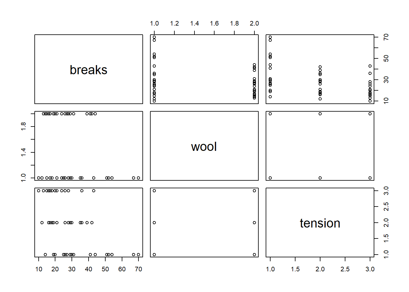
- Use the Poisson family and fit breaks with wool, tension, and their interaction.
pMod <- glm(breaks ~ wool * tension, family = poisson, data = warpbreaks)

summary(pMod)
##
## Call:
## glm(formula = breaks ~ wool * tension, family = poisson, data = warpbreaks)
##
## Deviance Residuals:
## Min 1Q Median 3Q Max
## -3.3383 -1.4844 -0.1291 1.1725 3.5153
##
## Coefficients:
## Estimate Std. Error z value Pr(>|z|)
## (Intercept) 3.79674 0.04994 76.030 < 2e-16 ***
## woolB -0.45663 0.08019 -5.694 1.24e-08 ***
## tensionM -0.61868 0.08440 -7.330 2.30e-13 ***
## tensionH -0.59580 0.08378 -7.112 1.15e-12 ***
## woolB:tensionM 0.63818 0.12215 5.224 1.75e-07 ***
## woolB:tensionH 0.18836 0.12990 1.450 0.147
## ---
## Signif. codes: 0 '***' 0.001 '**' 0.01 '*' 0.05 '.' 0.1 ' ' 1
##
## (Dispersion parameter for poisson family taken to be 1)
##
## Null deviance: 297.37 on 53 degrees of freedom
## Residual deviance: 182.31 on 48 degrees of freedom
## AIC: 468.97
##
## Number of Fisher Scoring iterations: 4- Check to see if this is an appropriate model. If not, choose a more appropriate model form.
1 - pchisq(deviance(pMod), df.residual(pMod))## [1] 0pMod2 <- glm(breaks ~ wool * tension,
family = "quasipoisson",
data = warpbreaks)
pMod2Diag <- data.frame(warpbreaks,
link = predict(pMod2, type = "link"),
fit = predict(pMod2, type = "response"),
pearson = residuals(pMod2, type = "pearson"),
resid = residuals(pMod2, type = "response"),
residSqr = residuals(pMod2, type = "response")^2
)
ggplot(pMod2Diag, aes(x = fit, y = residSqr)) +
geom_point() +
geom_abline(intercept = 0, slope = 1, size = 1) +
geom_abline(intercept = 0, slope = summary(pMod2)$dispersion,
color = "darkgreen", linetype = 2, size = 1) +
geom_smooth(se = F, size = 1) +
theme_bw() ## `geom_smooth()` using method = 'loess' and formula 'y ~ x'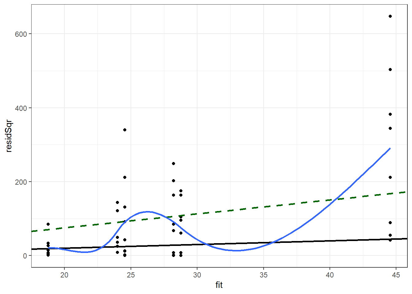
nbMod <- glm.nb(breaks ~ wool * tension,
                data = warpbreaks)

summary(nbMod)
##
## Call:
## glm.nb(formula = breaks ~ wool * tension, data = warpbreaks,
## init.theta = 12.08216462, link = log)
##
## Deviance Residuals:
## Min 1Q Median 3Q Max
## -2.09611 -0.89383 -0.07212 0.65270 1.80646
##
## Coefficients:
## Estimate Std. Error z value Pr(>|z|)
## (Intercept) 3.7967 0.1081 35.116 < 2e-16 ***
## woolB -0.4566 0.1576 -2.898 0.003753 **
## tensionM -0.6187 0.1597 -3.873 0.000107 ***
## tensionH -0.5958 0.1594 -3.738 0.000186 ***
## woolB:tensionM 0.6382 0.2274 2.807 0.005008 **
## woolB:tensionH 0.1884 0.2316 0.813 0.416123
## ---
## Signif. codes: 0 '***' 0.001 '**' 0.01 '*' 0.05 '.' 0.1 ' ' 1
##
## (Dispersion parameter for Negative Binomial(12.0822) family taken to be 1)
##
## Null deviance: 86.759 on 53 degrees of freedom
## Residual deviance: 53.506 on 48 degrees of freedom
## AIC: 405.12
##
## Number of Fisher Scoring iterations: 1
##
##
## Theta: 12.08
## Std. Err.: 3.30
##
## 2 x log-likelihood: -391.125- Use the backward selection method to reduce your model, if possible. Use your model from the prior problem as the starting model.
step(nbMod, test = "LRT")## Start: AIC=403.12
## breaks ~ wool * tension
##
## Df Deviance AIC LRT Pr(>Chi)
## <none> 53.506 403.12
## - wool:tension 2 61.712 407.33 8.206 0.01652 *
## ---
## Signif. codes: 0 '***' 0.001 '**' 0.01 '*' 0.05 '.' 0.1 ' ' 1##
## Call: glm.nb(formula = breaks ~ wool * tension, data = warpbreaks,
## init.theta = 12.08216462, link = log)
##
## Coefficients:
## (Intercept) woolB tensionM tensionH woolB:tensionM
## 3.7967 -0.4566 -0.6187 -0.5958 0.6382
## woolB:tensionH
## 0.1884
##
## Degrees of Freedom: 53 Total (i.e. Null); 48 Residual
## Null Deviance: 86.76
## Residual Deviance: 53.51 AIC: 405.1No terms can be dropped from the model.
- Check the residual variance assumption for your model.
nbModDiag <- data.frame(warpbreaks,
                        link = predict(nbMod, type = "link"),
                        fit = predict(nbMod, type = "response"),
                        pearson = residuals(nbMod,type = "pearson"),
                        resid = residuals(nbMod,type = "response"),
                        residSqr = residuals(nbMod,type = "response")^2
                        )

ggplot(nbModDiag, aes(x = fit, y = residSqr)) +
  geom_point() +
  geom_abline(intercept = 0, slope = 1, size = 1) +
  geom_abline(intercept = 0, slope = summary(pMod2)$dispersion,
              color="darkgreen", linetype = 2, size = 1) +
  stat_function(fun=function(fit) {fit + fit^2 / summary(nbMod)$theta},
                color="red", size = 1) +
  geom_smooth(se = F, size = 1) +
  theme_bw()
## `geom_smooth()` using method = 'loess' and formula 'y ~ x'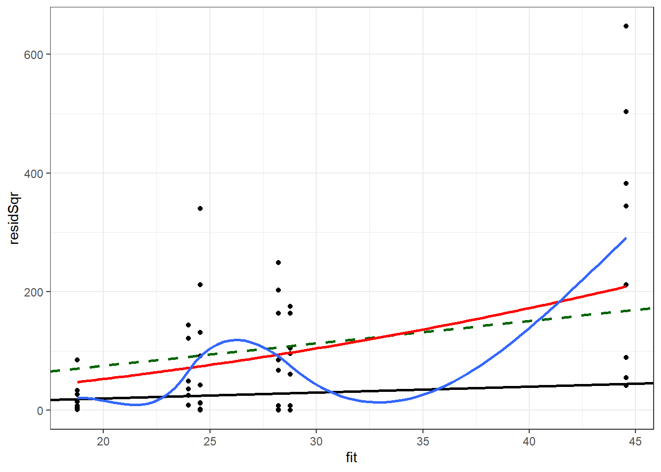
The negative binomial model is closer to means of the loess line than to the quasi-Poisson model. The range of values predicted by the model for the predicted values below 20 appears to be overstated by this model, though not as much as by the quasi-Possion model.