4 Outputs

Once we have user input, it is time to tell our app what to do with these values. One way of doing this is calling input objects within a render*() function.

4.1 render*() functions

Objects from input (created in ui) can be called and operated on within a render*() function and stored in output (in server), and then called with an *Output() function (in ui).

Each *Output() function is paired with a render*() function:

`render*()` function	`*Output()` function	Uses
`renderTable()`	`tableOutput()`	Simple tables
`renderDataTable()`	`dataTableOutput()`	Feature-rich tables with search, filter, and pagination
`renderImage()`	`imageOutput()`	Images
`renderPlot()`	`plotOutput()`	Plots
`renderPrint()`	`verbatimTextOutput()`	Text in the style of that returned by `print()`
`renderText()`	`textOutput()`	“Normal” text
`renderUI()`	`uiOutput()`, `htmlOutput()`	Dynamic outputs, HTML code

Examples of the first six pairs of render*() and *Output() functions can be seen in the app below. To see the source code, click here to view the full app.

4.2 Example App

The app produced by the code below allows users to filter the mtcars data by values of cyl, and then it plots the raw data and fits a simple regression. In practice, fitting models is not a good idea for Shiny apps. Even fairly basic models with small datasets can take minutes to fit, which is a long time for a user to wait for a webpage. Instead, try returning summary statistics such as means or ranges, or if you are set on returning regression results, have a few models pre-fit and saved as data files, and then read these in and display them in the app.

Copy the code below into a script and save it to run the app. Observe how renderPlot() is paired with plotOutput(), and renderText() with textOutput().

library(shiny)
library(dplyr)
library(ggplot2)

ui <-
  fluidPage(
    checkboxGroupInput("cyls",
                       "Number of cylinders:",
                       choices = c(4, 6, 8),
                       selected = c(4, 6, 8)),
    
    plotOutput(outputId = "myPlot"),
    
    textOutput(outputId = "myText")
  )

server <-
  function(input, output) {
    
    output$myPlot <-
      renderPlot({
        dat <- mtcars |> filter(cyl %in% input$cyls)
        coefs <- lm(mpg ~ wt, data = dat) |> coef()
        
        ggplot(dat, aes(wt, mpg)) +
          geom_point() +
          geom_abline(intercept = coefs[1], slope = coefs[2], linetype = 2)
      })
    
    output$myText <-
      renderText({
        dat <- mtcars |> filter(cyl %in% input$cyls)
        coefs <- lm(mpg ~ wt, data = dat) |> coef()
        
        paste("The line has intercept", 
              round(coefs[1], 2), 
              "and slope", 
              round(coefs[2], 2)
              )      
        })
    
  }

shinyApp(ui = ui, server = server, options = list(display.mode = "showcase"))

Note that instead of providing coefficients to geom_abline(), we could have had ggplot calculate the best fitting line for us with geom_smooth(method = "lm", se = F).

Also note that the render*() functions also have curly braces ({}) inside. They are only required if more than one expression is inside, but it is best practice to always include them. Here, both renderPlot() and renderText() each have three expressions (dat <- ..., coefs <- ..., and ggplot(... or paste(...), so they are required.

Each render*() function stores its result in output$outputId in server, and this is accessed by ui as just outputId within an *Output() function, such as how plotOutput() accesses output$myPlot with plotOutput("myPlot").

While this app works fine enough to produce a plot and return the intercept and slope of a simple linear regression, you may notice some problems with the app:

How many times did we filter the same data and fit the same model? (We will learn how to fix this in Reactivity.)
What happens if you uncheck all the options in the input? (We will revisit this in Error Messages.)

4.3 Responsive Inputs

The functions in the final line of the table above, renderUI() plus uiOutput() or htmlOutput(), can be used to create reactive outputs. uiOutput() is just an alias for htmlOutput(), so the two functions can be used interchangeably. One of their uses is to create inputs whose values change in response to another input.

You have probably encountered such inputs when filling out your address in an online form. A first question may have asked you to pick your state of residence from a menu, and then the second question asked you to pick your county. Depending on which state was selected, different values of county appeared in the second question.

Two examples of responsive inputs can be viewed below or by clicking here.

Let’s look at the parts of the app that were used to create the first input pair.

library(shiny)

ui <-
  fluidPage (
    radioButtons(inputId = "region",
                 label = "Pick a region of the US",
                 choices = levels(state.region)),
    
    uiOutput(outputId = "myUI")
  )

server <-
  function(input, output) {
    output$myUI <-
      renderUI({
        selectInput(inputId = "state", 
                    label = "Pick a state in that region:",
                    choices = state.name[state.region == input$region])
      })
  }

shinyApp(ui = ui, server = server, options = list(display.mode = "showcase"))

In this code, the value of input$region from radioButtons() in ui is passed to selectInput() within renderUI() in server. The input control is then returned to uiOutput() in ui. In contrast to the outputs we have previously seen, responsive outputs can be interacted with and pass their values onto other render*() functions.

The next step, then, would be to use the value of input$state in a render*() function, which would return an object to the output.

4.4 Character Data

Many *Input() functions return character vectors, and these can be tricky to use. In the app we created, selectInput() returns a character vector, and our plot call is plot(mtcars[, input$xvar], mtcars$mpg). Different extractors ([], $) require different data types.

4.4.1 Variables

For example, we can create a simple character vector with length one called x, and make its value "wt", one of the column names in mtcars. First note that we cannot extract mtcars$wt with mtcars$x. We must use the square brackets ([]). On the other hand, tidyselect functions like pull() or select() accept character vectors, so no special notation is needed.

library(dplyr)

x <- "wt"

mtcars$x

## NULL

mtcars[, x]

##  [1] 2.620 2.875 2.320 3.215 3.440 3.460 3.570 3.190 3.150 3.440 3.440 4.070
## [13] 3.730 3.780 5.250 5.424 5.345 2.200 1.615 1.835 2.465 3.520 3.435 3.840
## [25] 3.845 1.935 2.140 1.513 3.170 2.770 3.570 2.780

mtcars |> pull(x)

##  [1] 2.620 2.875 2.320 3.215 3.440 3.460 3.570 3.190 3.150 3.440 3.440 4.070
## [13] 3.730 3.780 5.250 5.424 5.345 2.200 1.615 1.835 2.465 3.520 3.435 3.840
## [25] 3.845 1.935 2.140 1.513 3.170 2.770 3.570 2.780

As we have already seen, to plot in base R, we should use square brackets rather than the dollar sign. For ggplot, the notation is a bit more complicated. ggplot requires variable names as aesthetics, so we need to tell ggplot that the character string is a column in our dataset with .data[[x]].

x <- "wt"
plot(mtcars$x, mtcars$mpg) # incorrect

## Error in xy.coords(x, y, xlabel, ylabel, log): 'x' and 'y' lengths differ

plot(mtcars[, x], mtcars$mpg) # correct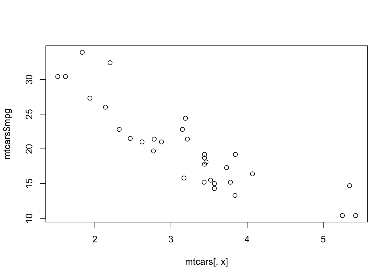

library(ggplot2)
ggplot(mtcars, aes(x, mpg)) + geom_point() # incorrect

ggplot(mtcars, aes(.data[[x]], mpg)) + geom_point() # correct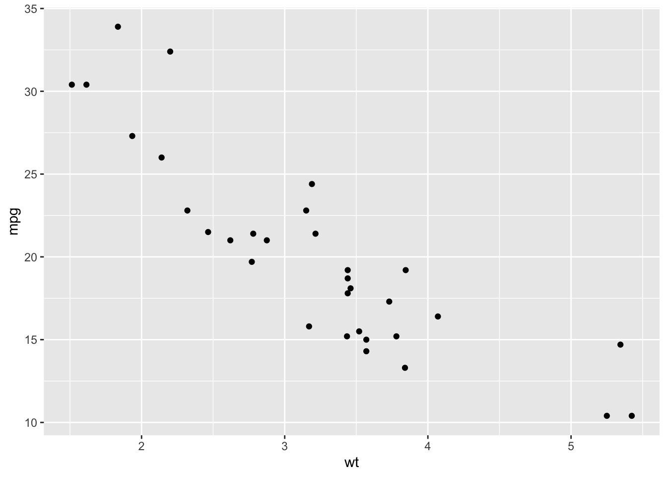

4.4.2 Formulas

lm() and other modeling functions also have special requirements that the formula argument must be of class formula, not of class character. To change the data type to formula, simply pass a character string to as.formula().

x <- "wt"
myFormula <- as.formula(paste("mpg ~", x))
myFormula

## mpg ~ wt

lm(myFormula, data = mtcars)

## 
## Call:
## lm(formula = myFormula, data = mtcars)
## 
## Coefficients:
## (Intercept)           wt  
##      37.285       -5.344

If one or more variables are to be supplied to a formula, as might be the case with checkboxGroupInput() (e.g., “Check the predictors to include in the model”), the collapse argument of paste() comes in handy. We can use collapse = "+" to take all the elements from x and combine them into a single element, inserting + between each one.

x <- c("wt", "hp", "disp")
myFormula <- as.formula(paste("mpg ~",
                              paste(x, collapse = "+")
                              )
                        )
myFormula

## mpg ~ wt + hp + disp

lm(myFormula, data = mtcars)

## 
## Call:
## lm(formula = myFormula, data = mtcars)
## 
## Coefficients:
## (Intercept)           wt           hp         disp  
##   37.105505    -3.800891    -0.031157    -0.000937

To see which data type a specific *Input() function returns, check the “Server value” section in the documentation.

4.5 Exercises

Check Your Understanding:

Copy and paste the following code into a new R script and save it. Click “Run App”. This app returns a plot of weight by MPG in the mtcars dataset, with weight filtered to be within a range picked by the user. Modify the app in these ways:

Add a table output of the filtered dataset.
Add a text output with summary statistics of mpg after filtering, such as its mean (mean()), standard deviation (sd()), or interquartile range (IQR()).

library(shiny)
library(dplyr)
library(ggplot2)

ui <- 
  fluidPage(
    sliderInput(inputId = "range", 
                label = "Pick a range for mtcars$wt", 
                min = 1.5,
                max = 5.5,
                value = c(1.5, 5.5)),
    
    plotOutput(outputId = "myPlot")
  )

server <-
  function(input, output) {
    output$myPlot <- 
      renderPlot({
        dat <- 
          mtcars |>
          filter(wt >= input$range[1], 
                 wt <= input$range[2]) 
        
        ggplot(dat, aes(wt, mpg)) +
          geom_point()
    })
    
  }

shinyApp(ui = ui, server = server)

Challenge:

Follow up on the idea in the end of the section on Responsive Inputs. Use the value of input$state in another output. Copy the code below into an R script and save it to create an app. Add a renderText() in server that returns a fact about the selected state (input$state) from the state.x77 dataset, such as its population, which you can retrieve with state.x77[input$state, "Population"]. Then, display this text with a textOutput() in ui.

library(shiny)

ui <-
  fluidPage (
    radioButtons("region",
                 "Pick a region of the US",
                 levels(state.region)),
    
    uiOutput(outputId = "myUI")
  )

server <-
  function(input, output) {
    output$myUI <-
      renderUI({
        selectInput(inputId = "state", 
                    label = "Pick a state in that region:",
                    choices = state.name[state.region == input$region])
      })
  }

shinyApp(ui = ui, server = server, options = list(display.mode = "showcase"))

Create Your Own App:

Continue to work on the app you started in the previous chapter’s exercises.

Use the values from the inputs created in the previous exercises in at least two render*() functions.
Create an output for each render*() function.
Run your app.