Mixed Models: Diagnostics and Inference
This article is part of the Mixed Model series. For a list of topics covered by this series, see the Introduction article. If you're new to mixed models we highly recommend reading the articles in order.
Overview
This article describes some of the some of the currently available diagnostic tools for mixed models. Also covered in this article are some additional inferences which can be made from mixed models.
Model diagnostics are typically done as models are being constructed. Model construction and diagnostics were split into separate articles for pedagogical purposes, but we recommend doing model diagnostics as models are being constructed.
Diagnostics
Mixed models add at least one random variable to a linear or generalized linear model. The random variables of a mixed model add the assumption that observations within a level, the random variable groups, are correlated. Mixed models are designed to address this correlation and do not cause a violation of the independence of observations assumption from the underlying model, e.g. linear or generalized linear. The assumption is relaxed to observations are independent of the other observations except where there is correlation specified by the random variable groups. There is also a new independence assumption for mixed models. This is the effects associated with the random variable groups are uncorrelated with the means of the fixed effect from the random variable groups. All other assumptions for mixed models are the same as the assumptions of the underlying model.
Model form diagnostics
An OLS model is assumed to be linear with respect to the predicted value with constant variance. A GLM model is assumed to be linear on the link scale. For some GLM models the variance of the Pearson's residuals is expected to be approximate constant. Residual plots are a useful tool to examine these assumptions on model form. The plot() function will produce a residual plot when the first parameter is a lmer() or glmer() returned object. The following code produces a residual plot for the mm model (constructed in the Models article of this series.)
Enter the following command in your script and run it.
plot(mm)The results of the above command are shown below.
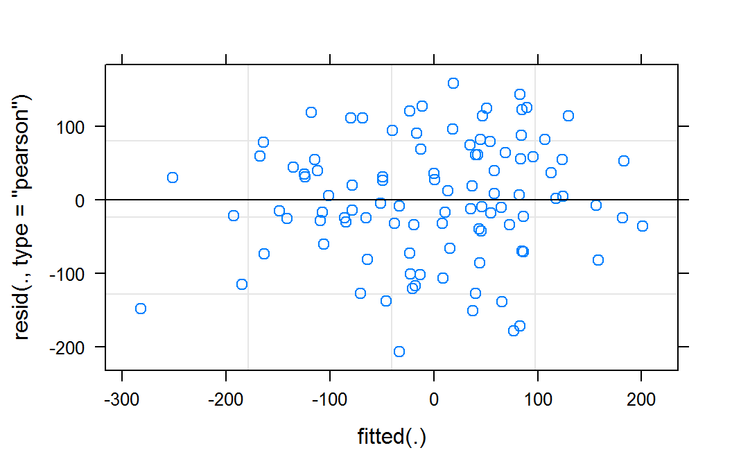
Residual plot of mm for lmer object
This residual plot does not indicate any deviations from a linear form. It also shows relatively constant variance across the fitted range. The slight reduction in apparent variance on the right and left of the graph are likely a result of there being fewer observation in these predicted areas.
The residual plot for a logistic model does not provide information on the appropriateness of the model form. They are typically not considered. For other generalized models the residual can assist in assessing the form of the model fit. We will produce a residual plot for our logistic example model to demonstrate how this is done for generalized model.
The plot() function will produce a residual plot for a glmm model that is similar to the plot for lmer models. The plot() function plots the Pearson residuals, residuals scaled by variance function, verses the fitted values on the response scale. For generalized models it is often more useful to examine the residuals plotted on the link scale, \(\eta\), instead of the response scale. The following code demonstrate producing a residual plot on the link scale.
Enter the following command in your script and run it.
ggplot(data.frame(eta=predict(gmm,type="link"),pearson=residuals(gmm,type="pearson")),
      aes(x=eta,y=pearson)) +
    geom_point() +
    theme_bw()
The results of the above command are shown below.
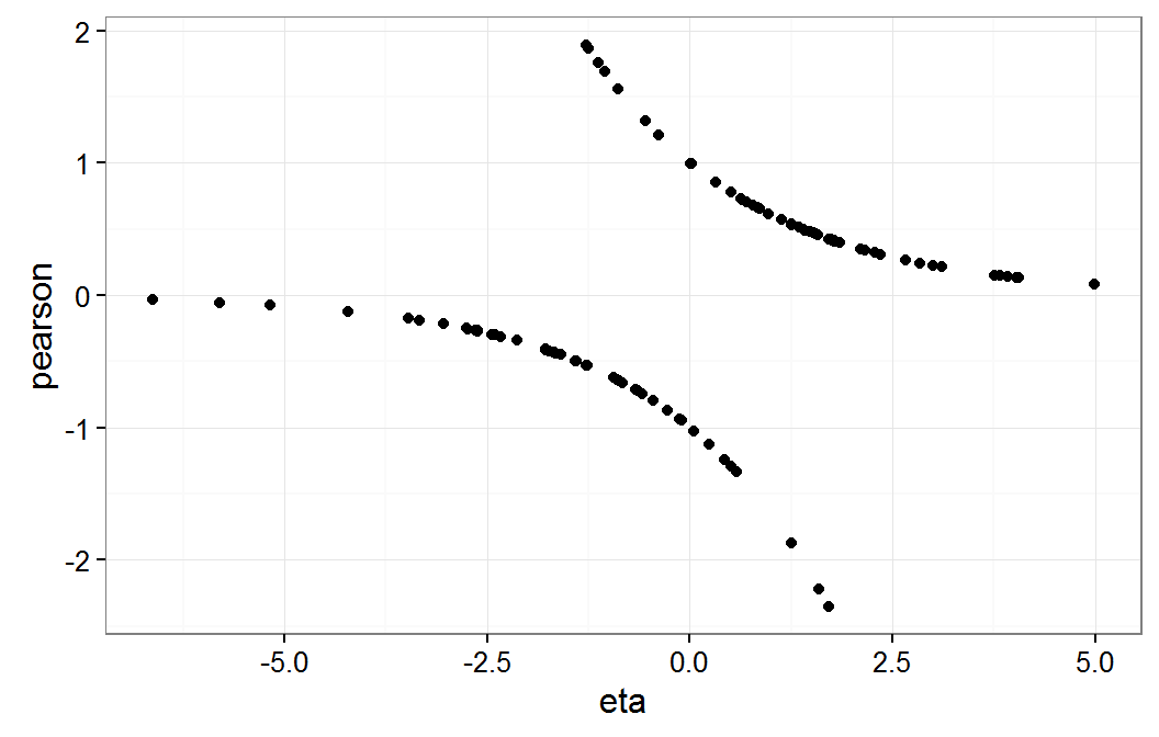
Residual plot of gmm on eta scale
As expected, this residual plot does not provide information about the model form assumptions for our dichotomous response logistic model.
Linearity in each variable
Models are assumed to be linear in each of the independent variables. This assumption can be checked with plots of the residuals versus each of the variables. The following code displays the residuals plotted to the x1 and x2 variables.
Enter the following commands in your script and run them.
ggplot(data.frame(x1=pbDat$x1,pearson=residuals(gmm,type="pearson")),
      aes(x=x1,y=pearson)) +
    geom_point() +
    theme_bw()

ggplot(data.frame(x2=pbDat$x2,pearson=residuals(gmm,type="pearson")),
      aes(x=x2,y=pearson)) +
    geom_point() +
    theme_bw()
The results of the above commands are shown below.
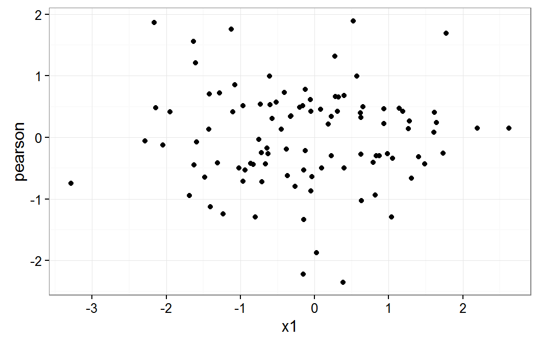
Residual plot on x1
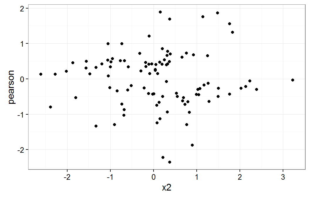
Residual plot on x2
These plot do not raise any concern about a non linear relationship for x1 or x2 variables.
The relationship to the g1 variable was not considered. The assumption for these random levels is that there will be differences in the means. There for we did not plot this relationship.
Independence
We will check if the group means of x1 and x2 are correlated with the g1 effects without the shrinkage of the mixed model applied. The following code extracts these values from the pbDat data frame and the model with g1 as a fixed effect. The correlation is then displayed.
Enter the following commands in your script and run them.
means <- aggregate(pbDat[,c("x1","x2")],by=list(pbDat$g1),FUN=mean)
lmcoefs <- summary(lm(y ~ x1 + x2 + g1, data=pbDat))$coefficients[,"Estimate"]
means$effects <- c(0,lmcoefs[substr(names(lmcoefs),1,2) == "g1"])
means$effects <- means$effects - mean(means$effects)

cor(means[,c("x1","x2","effects")])
The results of the above commands are shown below.
                 x1         x2    effects
x1       1.00000000 0.01851362 -0.3338548
x2       0.01851362 1.00000000  0.6687850
effects -0.33385483 0.66878500  1.0000000
We see that both x1 and x2 are moderately correlated, -0.3338548 and 0.668785, with the g1 effects.
The following plots graphically display this correlation.
Enter the following commands in your script and run them.
ggplot(means, aes(x=x1,y=effects)) +
    geom_point() +
    theme_bw()

ggplot(means, aes(x=x2,y=effects)) +
    geom_point() +
    theme_bw()
There are no console results from these commands. The following plot is produced.
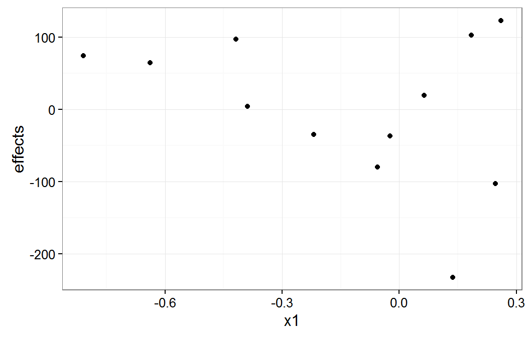
plot of x1 group means

plot of x2 group means
The x1 plot shows that the groups with effect values of about -100 and -200 are the source of most of the correlation between x1 and g1. The x2 plot shows that it group with the effect value of about -200 is the source of the correlation between x2 and g1.
This correlation may bias the estimates of the fixed effects. The follow code displays the estimated fixed effects from the mm model and the same effects from the model which uses g1 as a fixed effect.
Enter the following commands in your script and run them.
fixef(mm)
lmcoefs[1:3]
The results of the above commands are shown below.
(Intercept)          x1          x2
   3.240341   17.660738  -55.430494
(Intercept) x1 x2 100.51251 18.26735 -57.60793
The coefficient values for x1 and x2 changed by less than 5 percent. One would need to decide based on the science of the analysis being done if this is a meaningful change in the coefficient.
Normality of residuals
Normality of the residuals is typically checked with with a q-q plot (quantile-quantile.) Significant deviations from linearity of the observations or non-symmetric scales indicate a deviation from normality of the residuals.
Enter the following command in your script and run it.
qqnorm(residuals(mm))There are no console results from this command. The following plot is produced.
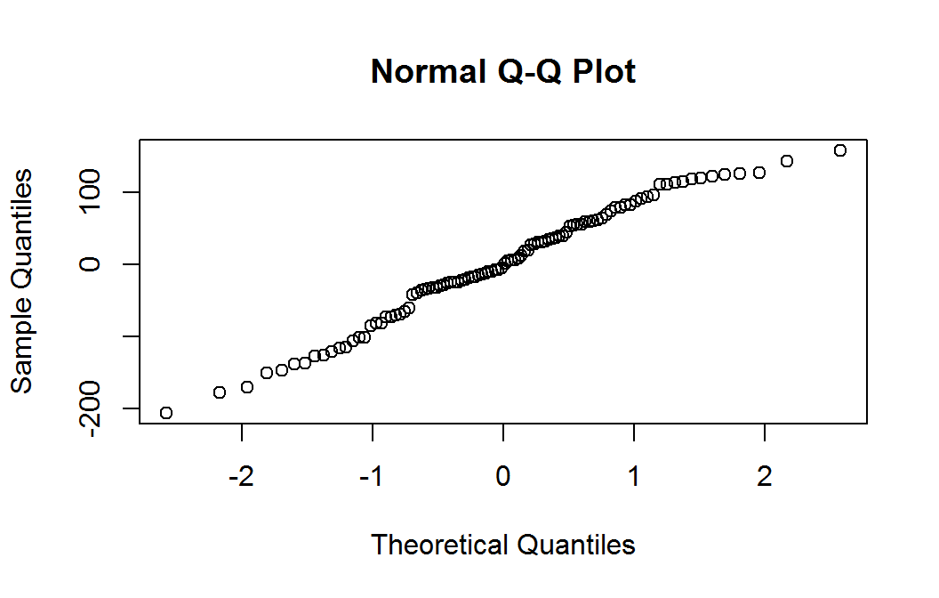
Residual nrmal probability plot
The quantile plot (also called a normal probability plot) does not raise any significant concern with normality of the weighted residuals.
Sensitivity to data
It is important to check that your model is not influenced by one or a small set of observations. This might indicate your model is over fit or that your model is sensitive to the particular observations included in the model. Typical tools for measuring leverage and influence are limited for mixed models. This is due to these concepts not transferring from linear and generalized linear models to mixed models. The one tool we have is leverage for linear mixed models.
Mixed models work by providing some shrinkage to the random effects, this is the \(\boldsymbol{b}\)s in the \(Y \, | \, \boldsymbol{B}=\boldsymbol{b} \ \ \sim \ \ N(\boldsymbol{X\beta} + \boldsymbol{Z b}, \sigma^2 \boldsymbol{I})\) model. Compared to their values as \(\boldsymbol{\beta}\)s as fixed effects, the \(\boldsymbol{b}\)s are shrunk towards zero, which would be the same as not including the effects in the model as either a fixed or random variable. The shrinkage amount is based on how much information is contained in a random effect groups. This can be used to get a look at what what observations may be stressing the model. This would be done by creating both the fixed effect model and the model with the random effects completely dropped. These will be either linear or generalized linear models. Evaluate both of these models for observations which have high leverage and/or high Cook's distance. Then evaluate the change in the coefficients in the mixed model by dropping the observations which were identified by the linear or generalized model. See the Regression Diagnostics article for instructions and examples on identifying leverage and Cook's distance in linear and generalized linear models.
The following code generates a plot of the leverage (hatvalues) verse the Pearson residuals.
Enter the following command in your script and run it.
ggplot(data.frame(lev=hatvalues(mm),pearson=residuals(mm,type="pearson")),
      aes(x=lev,y=pearson)) +
    geom_point() +
    theme_bw()
The results of the above command are shown below.
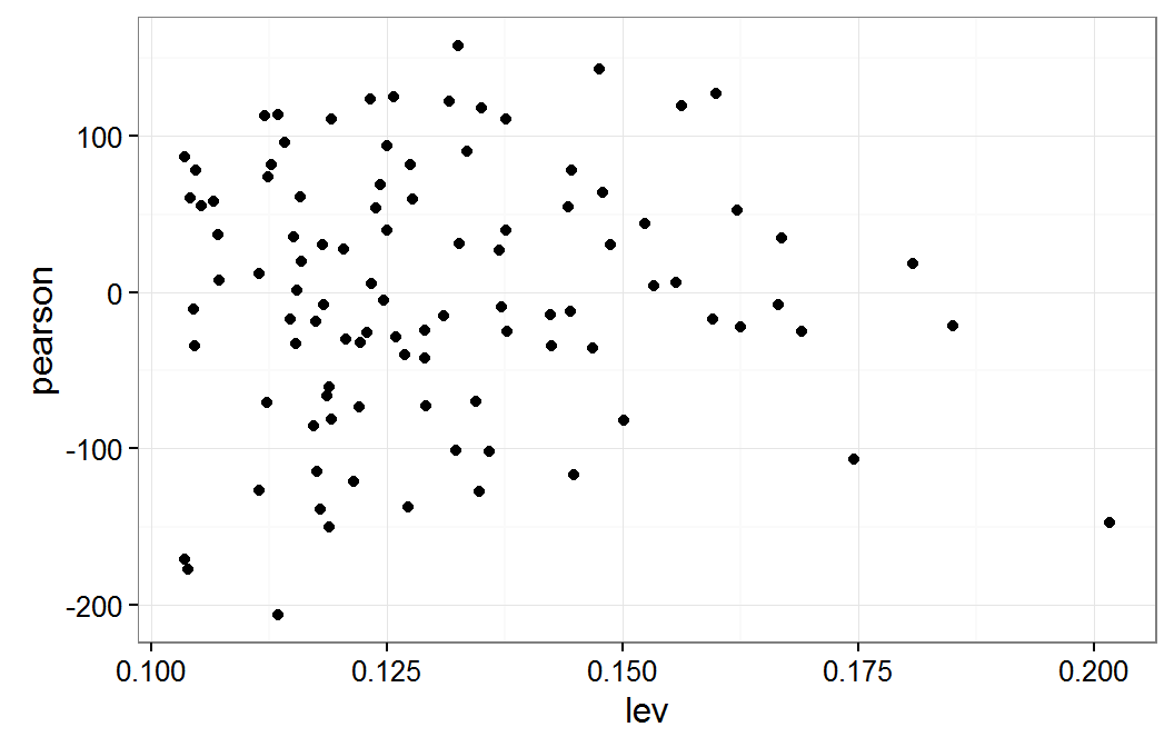
Residual plot verse leverage for mm model
The following code determines which of the observations have the highest leverage and displays these observations. The code also generates a new model without these observations and then compares the coefficients for the will all observations to this new model with some observations removed.
Enter the following command in your script and run it.
levId <- which(hatvalues(mm) >= .172)
pbDat[levId,c("y","x1","x2","g1")]
summary(pbDat[,c("y","x1","x2")])

mmLev <- lmer(y ~ x1 + x2 + (1|g1), data=pbDat[-c(levId),])
mmLevCD <- data.frame(effect=fixef(mm),
                     change=(fixef(mmLev) - fixef(mm)),
                     se=sqrt(diag(vcov(mm)))
                     )
rownames(mmLevCD) <- names(fixef(mmLev))
mmLevCD$multiples <- abs(mmLevCD$change / mmLevCD$se)
mmLevCD
The results of the above command are shown below.
            y        x1          x2 g1
5   -98.06299 -3.286493  0.07252566  E
42   55.73686 -2.144218 -0.98229879  F
93 -214.17818 -2.290438  2.22630416  I
72 -429.90495 -0.750835  3.21873091  L
y x1 x2 Min. :-429.905 Min. :-3.2865 Min. :-2.61004 1st Qu.: -95.839 1st Qu.:-0.8813 1st Qu.:-0.68087 Median : 3.828 Median :-0.1438 Median : 0.14794 Mean : -2.412 Mean :-0.1418 Mean : 0.09448 3rd Qu.: 104.556 3rd Qu.: 0.6261 3rd Qu.: 0.77479 Max. : 243.756 Max. : 2.6189 Max. : 3.21873effect change se multiples (Intercept) 3.240341 2.503425 29.815555 0.08396373 x1 17.660738 -4.585005 8.316416 0.55131984 x2 -55.430494 6.015218 8.602384 0.69925012
These results show that observations 5, 42, 93, and 72 have the highest leverage values. We can also see that either the x1 or x2 variable values are outside of their interquartile range (IQR.) For some of these observations both x1 and x2 are outside their IQR. When these observations are dropped from the model, the value of the coefficients change by one half and two thirds of a standard error. The science of the analysis would be used to determine if this amount of change is a cause for concern or not.
Exercises
Use the models from sleepstudy data set for the following exercises.
Create a residual plot for your linear sleep study model, the model from exercise 5 in the Models article.
Check the normality of the residuals from your linear sleep study model.
Check if your linear sleep study model has any leverage points of concern.
Additional inferences
Predictions
The response variable for a mixed model is of the form \((Y \, | \, B = b)\), as explained in the Models article. Predictions can be made for observations which are members of the observed levels of the random variables. This is a group level needs to be specified for each group defined in the random formula for the model. Since particular levels of random effects are not formal estimates of the model, care needs to be used when interpreting predicted values based on these levels.
The model results include an estimate of the mean value for each population represented by groups in the random portion of the model formula. These estimates of population means are incorporated in the fixed portion of the model. Predictions can also be made for these mean values. This is done by setting the re.form parameter of the predict() function to NA. These estimated means are formally estimated by the model and can be directly interpreted.
The predict() function does not produce a standard error for the predictions. This is due in part to the lack of a standard error for the estimated variance of the unobserved variables. If one was willing to make an assumptions about the variance, a parametric bootstrap could be used to produce a prediction intervals or confidence intervals.
We will use the predict function to estimate the predicted values for x1 = .5 at x2 = -.5 and x1 = -2 at x2 = .25. These will be estimates at the mean value of the unobserved random variable which was sampled at the level in variable g1. We then predict the response for these same two observations at the g1 level of "B". These predictions will be made on both the link scale (log odds for our gmm model) and the response scale (as probabilities.) The following code calculates these predictions.
Enter the following commands in your script and run them.
newDat <- data.frame(x1=c(.5,-2),x2=c(-.5,.25))
predict(gmm,newDat,re.form=NA,type="link")
predict(gmm,newDat,re.form=NA,type="response")
The results of the above commands are shown below.
        1         2
 1.172611 -1.212977
1 2 0.7636167 0.2291748Enter the following commands in your script and run them.
newDat2 <- data.frame(x1=c(.5,-2),x2=c(-.5,.25),g1=c("B","B"))
predict(gmm,newDat2,type="link")
predict(gmm,newDat2,type="response")
The results of the above commands are shown below.
         1          2
 1.8154964 -0.5700918
1 2 0.8600248 0.3612156
Inter Class Correlation (ICC)
ICC is a measure of how much of the variation in the response variable, which is not attributed to fixed effects, is accounted for by a random effect. It is the ratio of the variance of the random effect to the total random variation. The code to calculate the ICC for the mm model is demonstrated here.
Enter the following commands in your script and run them.
r1Var <- as.numeric(VarCorr(mm)[["g1"]])
residVar <- attr(VarCorr(mm), "sc")^2
r1Var
residVar
r1Var / (r1Var + residVar)
The results of the above commands are shown below.
[1] 9736.123
[1] 7564.864
[1] 0.5627496
This would be interpreted as 56 percent of the stochastic variation is accounted for by g1.
For the generalized model, the residual variance is a known constant. We will use \((15/16)^2 \pi^2 / 3\) as an estimate of the variance of the logistic distribution.
Enter the following commands in your script and run them.
r1Var <- as.numeric(VarCorr(gmm)[["g1"]])
residVar <- (15/16)^2 * pi^2 / 3
r1Var
residVar
r1Var / (r1Var + residVar)
The results of the above commands are shown below.
[1] 4.255377
[1] 2.891486
[1] 0.5954189
The g1 variable accounts for 60 percent of the stochastic variation in the gmm model.
Exercises
Use the models from sleepstudy data set for the following exercises.
- Predict the average response time for eight days in the sleep deprivation study. The model from exercise 5 in the Models article.
Previous: Testing Significance of Effects
Next: Multiple Random Parameters
Last Revised: 3/30/2016